Journal of Electromagnetic Analysis and Applications, 2012, 4, 513-522
http://dx.doi.org/10.4236/jemaa.2012.412072 Published Online December 2012 (http://www.SciRP.org/journal/jemaa)
513
Electromagnetic Response Studies of the Antenna for Deep
Water Deep Target CSEM Environments
Noorhana Yahya1, Nadeem Nasir2,3, Majid Niaz Akhtar2,4, Muhammad Kashif2, Tanvir Hussain5,
Hasnah Mohd Zaid1, Afza Shafie1
1Fundamental and Applied Science Department, Tronoh, Malayia; 2Electrical and Electronic Engineering Department, Tronoh, Malayia;
3Fundamental and Applied Science Department, National Textile University, Faisalabad, Pakistan; 4Comsats Institute of Information
Technology Lahore, Lahore, Pakistan; 5Mechanical Engineering Department, Universiti Teknologi PETRONAS, Tronoh, Malaysia.
Received September 2nd, 2012; revised October 5th, 2012; accepted October 15th, 2012
ABSTRACT
The Controlled Source Electromagnetic Method (CSEM) is used for offshore hydrocarbon exploration. Hydrocarbon
detection in seabed logging (SBL) is a very challenging task for deep hydrocarbon reservoirs. The electromagnetic field
response of an antenna is unable to detect deep hydrocarbon reservoirs due to a weak electromagnetic signal response in
the seabed logging environment. This work premise deals with the comparison of the electromagnetic signal strength of
a new antenna with a straight antenna and the orientation of an antenna for deep target hydrocarbon exploration. An-
tenna position and orientation (Tx and Ty) was studied using Computer Simulation Technology software (CST) for deep
targets in marine CSEM environments. The model area was assigned as (40  40 km) to replicate the real seabed envi-
ronment. From the results, the new dipole antenna shows an 804% and 278% increase in electric and magnetic field
strength than the straight antenna. An electric (E) and magnetic (H) field component study was done with and without
the presence of a hydrocarbon reservoir. Ex and Hz field component responses with the new antenna at the 1 km target
were measured in a deep water environment. It was analyzed that the antenna shows 53.10% (Ex) and 83.13% (Hz) field
difference in deep water with and without a hydrocarbon reservoir at the 30 m antenna position from the sea floor. From
the antenna orientation results, it was observed that, the electric field Ex and magnetic field Hz responses decreased from
18% to 12% and 21% to 16%, respectively but was still able to detect the deep target hydrocarbon reservoir at the 4 km
target depth. This EM antenna may open new frontiers for the oil and gas industry for deep target hydrocarbon detection
(HC).
Keywords: Control Source Electromagnetic (CSEM); Seabed Logging (SBL); Antenna; Computer Simulation
Technology (CST); Hydrocarbon (HC)
1. Introduction
Seabed logging is an application of the control source
electromagnetic method which is used to locate an oil
reservoir beneath the sea floor by measuring electro-
magnetic fields [1-4]. Typically, in the control source
method, a horizontal electric dipole antenna is towed by
a surface vessel at a short distance from the sea floor [5-
7]. The dipole antenna transmits very low frequency
electromagnetic waves with frequencies ranging from
0.25 Hz - 10 Hz; due to the low frequency, transmitted
energy propagates down through the subsurface [8-10].
Low frequency electromagnetic waves attenuate more in
the conductive layer and less in the resistance layer due
to the skin depth. In a large resistive layer such as hy-
drocarbon, electromagnetic energy flows along the re-
servoir (described as a guided wave) and is detected by
the stationary sea floor electric or magnetic field detec-
tors which are deployed on the sea floor. The control
source electromagnetic method depends on the resistivity
of the hydrocarbon and the surrounding sediments. Hy-
drocarbon in the seabed has resistivity of a few tens to
hundred ohm meter (30 Ωm - 500 Ωm), sea water (0.5
Ωm - 2 Ωm) while all other layers including sediments in
the sea have resistivity of (1 Ωm - 2 Ωm) [11-18]. A 1D
numerical model for a marine CSEM environment with
the change of water depth and change of frequency was
reported [19]. His proposed model consists of a 1 km-
deep target depth, with a sea water layer of (0.3 Ωm)
over a (1 Ωm) half-space. A 100 m thick, 100-Ohm-m re-
sistive layer representing a hydrocarbon reservoir is em-
bedded at 1km below the seafloor for the 1D reservoir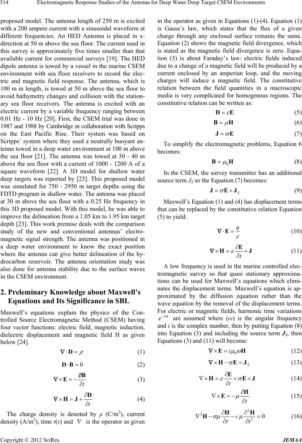

Electromagnetic Response Studies of the Antenna for Deep Water Deep Target CSEM Environments
514
proposed model. The antenna length of 250 m is excited
with a 200 ampere current with a sinusoidal waveform at
different frequencies. An HED Antenna is placed in x-
direction at 50 m above the sea floor. The current used in
this survey is approximately five times smaller than that
available current for commercial surveys [19]. The HED
dipole antenna is towed by a vessel in the marine CSEM
environment with sea floor receivers to record the elec-
tric and magnetic field response. The antenna, which is
100 m in length, is towed at 50 m above the sea floor to
avoid bathymetry changes and collision with the station-
ary sea floor receivers. The antenna is excited with an
electric current by a variable frequency ranging between
0.01 Hz - 10 Hz [20]. First, the CSEM trial was done in
1987 and 1988 by Cambridge in collaboration with Scripps
on the East Pacific Rise. Their system was based on
Scripps’ system where they used a neutrally buoyant an-
tenna towed in a deep water environment at 100 m above
the sea floor [21]. The antenna was towed at 30 - 40 m
above the sea floor with a current of 1000 - 1200 A of a
square waveform [22]. A 3D model for shallow water
deep targets was reported by [23]. This proposed model
was simulated for 750 - 2950 m target depths using the
FDTD program in shallow water. The antenna was placed
at 30 m above the sea floor with a 0.25 Hz frequency in
this 3D proposed model. With this model, he was able to
improve the delineation from a 1.05 km to 1.95 km target
depth [23]. This work premise deals with the comparison
study of the new and conventional antennas’ electro-
magnetic signal strength. The antenna was positioned in
a deep water environment to know the exact position
where the antenna can give better delineation of the hy-
drocarbon reservoir. The antenna orientation study was
also done for antenna stability due to the surface waves
in the CSEM environment.
2. Preleminary Knowledge about Maxwell’s
Equations and Its Significance in SBL
Maxwell’s equations explain the physics of the Con-
trolled Source Electromagnetic Method (CSEM) having
four vector functions: electric field, magnetic induction,
dielectric displacement and magnetic field H as given
below [24].

D (1)
0DB (2)
t


B
E

 (3)
t



D
HJ (4)
The charge density is denoted by ρ (C/m3), current
density (A/m2), time t(s) and

is the operator as given
in the operator as given in Equations (1)-(4). Equation (1)
is Gauss’s law, which states that the flux of a given
charge through any enclosed surface remains the same.
Equation (2) shows the magnetic field divergence, which
is stated as the magnetic field divergence is zero. Equa-
tion (3) is about Faraday’s law: electric fields induced
due to a change of a magnetic field will be produced by a
current enclosed by an amperian loop, and the moving
charges will induce a magnetic field. The constitutive
relation between the field quantities in a macroscopic
media is very complicated for homogenous regions. The
constitutive relation can be written as:


DE (5)


BH (6)


JE (7)
To simplify the electromagnetic problems, Equation 6
becomes:
0


BH (8)
In the CSEM, the survey transmitter has an additional
source term JS so the Equation (7) becomes:
S


JEJ (9)
Maxwell’s Equation (1) and (4) has displacement terms
that can be replaced by the constitutive relation Equation
(5) to yield:
q


E (10)
t





E
HJ
(11)
A low frequency is used in the marine controlled elec-
tromagnetic survey so that quasi stationary approxima-
tions can be used for Maxwell’s equations which elimi-
nates the displacement terms. Maxwell’s equation is ap-
proximated by the diffusion equation rather than the
wave equation by the removal of the displacement terms.
For electric or magnetic fields, harmonic time variations
t
e

  are assumed where (ω) is the angular frequency
and i is the complex number, then by putting Equation (8)
into Equation (3) and including the source term JS, then
Equations (3) and (11) will become:
0
i



EH

(12)
S


HEJ

(13)
t



 

E
HEJ (14)
t


 
H
E (15)
2
2
20
tt
 




HH
H
  (16)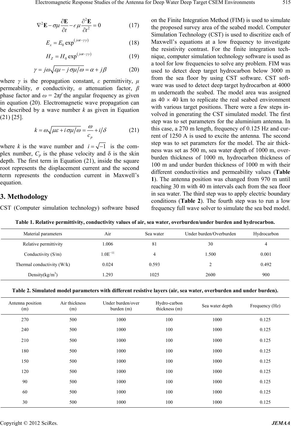

Electromagnetic Response Studies of the Antenna for Deep Water Deep Target CSEM Environments
515
on the Finite Integration Method (FIM) is used to simulate
the proposed survey area of the seabed model. Computer
Simulation Technology (CST) is used to discritize each of
Maxwell’s equations at a low frequency to investigate
the resistivity contrast. For the finite integration tech-
nique, computer simulation technology software is used as
a tool for low frequencies to solve any problem. FIM was
used to detect deep target hydrocarbon below 3000 m
from the sea floor by using CST software. CST soft-
ware was used to detect deep target hydrocarbon at 4000
m underneath the seabed. The model area was assigned
as 40  40 km to replicate the real seabed environment
with various target positions. There were a few steps in-
volved in generating the CST simulated model. The first
step was to set parameters for the aluminium antenna. In
this case, a 270 m length, frequency of 0.125 Hz and cur-
rent of 1250 A is used to excite the antenna. The second
step was to set parameters for the model. The air thick-
ness was set as 500 m, sea water depth of 1000 m, over-
burden thickness of 1000 m, hydrocarbon thickness of
100 m and under burden thickness of 1000 m with their
different conductivities and permeability values (Table
1). The antenna position was changed from 970 m until
reaching 30 m with 40 m intervals each from the sea floor
in sea water. The third step was to apply electric boundary
conditions (Table 2). The fourth step was to run a low
frequency full wave solver to simulate the sea bed model.
2
2
20
tt
 

 

EE
E  (17)

0exp

j
ty
x
EE

 
 (18)

0exp

j
ty
Z
HH

 
 (19)
jj j

   (20)
where γ is the propagation constant, ε permittivity, μ
permeability, σ conductivity, α attenuation factor, β
phase factor and ω = 2πf the angular frequency as given
in equation (20). Electromagnetic wave propagation can
be described by a wave number k as given in Equation
(21) [25].
p
ki
ci


    (21)
where k is the wave number and 1i is the com-
plex number, Cр is the phase velocity and  is the skin
depth. The first term in Equation (21), inside the square
root represents the displacement current and the second
term represents the conduction current in Maxwell’s
equation.
3. Methodology
CST (Computer simulation technology) software based
Table 1. Relative permittivity, conductivity values of air, sea water, overburde n/unde r burden and hydr oc arbon.
Material parameters Air Sea water Under burden/Overburden Hydrocarbon
Relative permittivity 1.006 81 30 4
Conductivity (S/m) 1.0E−11 4 1.500 0.001
Thermal conductivity (W/k) 0.024 0.593 2 0.492
Density(kg/m3) 1.293 1025 2600 900
Table 2. Simulated model parameters with different resistive layers (air, sea water, overburden and under burden).
Antenna position
(m)
Air thickness
(m)
Under burden/over
burden (m)
Hydro-carbon
thickness (m) Sea water depth Frequency (Hz)
270 500 1000 100 1000 0.125
240 500 1000 100 1000 0.125
210 500 1000 100 1000 0.125
180 500 1000 100 1000 0.125
150 500 1000 100 1000 0.125
120 500 1000 100 1000 0.125
90 500 1000 100 1000 0.125
60 500 1000 100 1000 0.125
30 500 1000 100 1000 0.125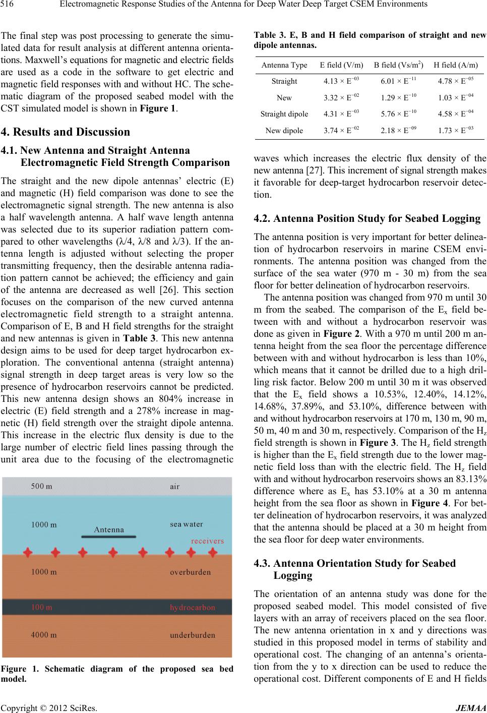

Electromagnetic Response Studies of the Antenna for Deep Water Deep Target CSEM Environments
516
The final step was post processing to generate the simu-
lated data for result analysis at different antenna orienta-
tions. Maxwell’s equations for magnetic and electric fields
are used as a code in the software to get electric and
magnetic field responses with and without HC. The sche-
matic diagram of the proposed seabed model with the
CST simulated model is shown in Figure 1.
4. Results and Discussion
4.1. New Antenna and Straight Antenna
Electromagnetic Field Strength Comparison
The straight and the new dipole antennas’ electric (E)
and magnetic (H) field comparison was done to see the
electromagnetic signal strength. The new antenna is also
a half wavelength antenna. A half wave length antenna
was selected due to its superior radiation pattern com-
pared to other wavelengths (λ/4, λ/8 and λ/3). If the an-
tenna length is adjusted without selecting the proper
transmitting frequency, then the desirable antenna radia-
tion pattern cannot be achieved; the efficiency and gain
of the antenna are decreased as well [26]. This section
focuses on the comparison of the new curved antenna
electromagnetic field strength to a straight antenna.
Comparison of E, B and H field strengths for the straight
and new antennas is given in Table 3. This new antenna
design aims to be used for deep target hydrocarbon ex-
ploration. The conventional antenna (straight antenna)
signal strength in deep target areas is very low so the
presence of hydrocarbon reservoirs cannot be predicted.
This new antenna design shows an 804% increase in
electric (E) field strength and a 278% increase in mag-
netic (H) field strength over the straight dipole antenna.
This increase in the electric flux density is due to the
large number of electric field lines passing through the
unit area due to the focusing of the electromagnetic
Figure 1. Schematic diagram of the proposed sea bed
model.
Table 3. E, B and H field comparison of straight and new
dipole antennas.
Antenna TypeE field (V/m)B field (Vs/m2) H field (A/m)
Straight 4.13 × E−03 6.01 × E−11 4.78 × E−05
New 3.32 × E−02 1.29 × E−10 1.03 × E−04
Straight dipole4.31 × E−03 5.76 × E−10 4.58 × E−04
New dipole 3.74 × E−02 2.18 × E−09 1.73 × E−03
waves which increases the electric flux density of the
new antenna [27]. This increment of signal strength makes
it favorable for deep-target hydrocarbon reservoir detec-
tion.
4.2. Antenna Position Study for Seabed Logging
The antenna position is very important for better delinea-
tion of hydrocarbon reservoirs in marine CSEM envi-
ronments. The antenna position was changed from the
surface of the sea water (970 m - 30 m) from the sea
floor for better delineation of hydrocarbon reservoirs.
The antenna position was changed from 970 m until 30
m from the seabed. The comparison of the Ex field be-
tween with and without a hydrocarbon reservoir was
done as given in Figure 2. With a 970 m until 200 m an-
tenna height from the sea floor the percentage difference
between with and without hydrocarbon is less than 10%,
which means that it cannot be drilled due to a high dril-
ling risk factor. Below 200 m until 30 m it was observed
that the Ex field shows a 10.53%, 12.40%, 14.12%,
14.68%, 37.89%, and 53.10%, difference between with
and without hydrocarbon reservoirs at 170 m, 130 m, 90 m,
50 m, 40 m and 30 m, respectively. Comparison of the Hz
field strength is shown in Figure 3. The Hz field strength
is higher than the Ex field strength due to the lower mag-
netic field loss than with the electric field. The Hz field
with and without hydrocarbon reservoirs shows an 83.13%
difference where as Ex has 53.10% at a 30 m antenna
height from the sea floor as shown in Figure 4. For bet-
ter delineation of hydrocarbon reservoirs, it was analyzed
that the antenna should be placed at a 30 m height from
the sea floor for deep water environments.
4.3. Antenna Orientation Study for Seabed
Logging
The orientation of an antenna study was done for the
proposed seabed model. This model consisted of five
layers with an array of receivers placed on the sea floor.
The new antenna orientation in x and y directions was
studied in this proposed model in terms of stability and
operational cost. The changing of an antenna’s orienta-
tion from the y to x direction can be used to reduce the
operational cost. Different components of E and H fields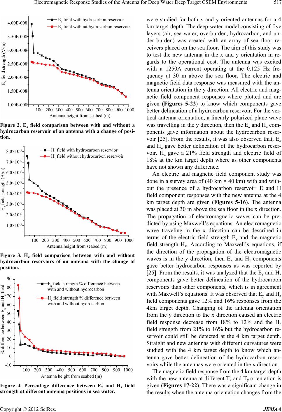

Electromagnetic Response Studies of the Antenna for Deep Water Deep Target CSEM Environments 517
Figure 2. Ex field comparison between with and without a
hydrocarbon reservoir of an antenna with a change of posi-
tion.
Figure 3. Hz field comparison between with and without
hydrocarbon reservoirs of an antenna with the change of
position.
Figure 4. Percentage difference between Ex and Hz field
strength at different antenna positions in sea water.
were studied for both x and y oriented antennas for a 4
km target depth. The deep-water model consisting of five
layers (air, sea water, overburden, hydrocarbon, and un-
der burden) was created with an array of sea floor re-
ceivers placed on the sea floor. The aim of this study was
to test the new antenna in the x and y orientation in re-
gards to the operational cost. The antenna was excited
with a 1250A current operating at the 0.125 Hz fre-
quency at 30 m above the sea floor. The electric and
magnetic field data response was measured with the an-
tenna orientation in the y direction. All electric and mag-
netic field component responses where plotted and are
given (Figures 5-22) to know which components gave
better delineation of a hydrocarbon reservoir. For the ver-
tical antenna orientation, a linearly polarized plane wave
was travelling in the y direction, then the Ex and Hz com-
ponents gave information about the hydrocarbon reser-
voir [25]. From the results, it was also observed that, Ex
and Hz gave better delineation of the hydrocarbon reser-
voir. Hz gave a 21% field strength and electric field of
18% at the km target depth where as other components
have not shown any difference.
An electric and magnetic field component study was
done in a survey area of (40 km × 40 km) with and with-
out the presence of a hydrocarbon reservoir. E and H
field component responses with the new antenna at the 4
km target depth are given (Figures 5-16). The antenna
was placed at 30 m above the sea floor in the x direction.
The propagation of electromagnetic waves can be pre-
dicted by using Maxwell’s equations. An electromagnetic
wave traveling in the x direction can be described in
terms of the electric field strength Ey and the magnetic
field strength Hz. According to Maxwell’s equations, if
the direction of the propagation of the electromagnetic
waves is in the y direction, then Ex and Hz components
gave better hydrocarbon responses as was reported by
[25]. From the results, it was analyzed that the Ey and Hz
components gave better delineation of the hydrocarbon
reservoirs than other components, which is in agreement
with Maxwell’s equations. It was observed that Ey and Hz
field components gave 12% and 16% responses from the
4km target depth. Changing of the antenna orientation
from the y direction to the x direction caused an electric
field response decrease from 18% to 12% and the Hz
field strength from 21% to 16% but the hydrocarbon re-
servoir could still be detected at the 4 km target depth.
Straight and new antennas with different curvatures were
studied with the 4 km target depth to know which an-
tenna gave better delineation of the hydrocarbon reser-
voirs while the antennas were oriented in the x direction.
The magnetic field response from the 4 km target depth
with the new antenna at different Tx and Ty orientation is
given (Figures 17-22). There was a significant change in
the results when the antenna orientation changes from the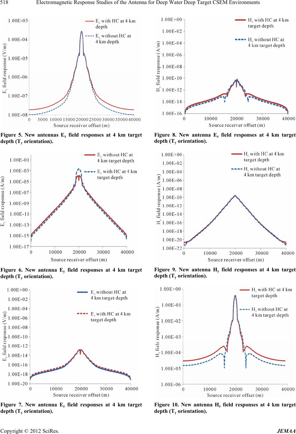

Electromagnetic Response Studies of the Antenna for Deep Water Deep Target CSEM Environments
518
Figure 5. New antennas Ex field responses at 4 km target
depth (Ty orientation).
Figure 6. New antenna Ey field responses at 4 km target
depth (Ty orientation).
Figure 7. New antenna Ez field responses at 4 km target
depth (Ty orientation).
Figure 8. New antenna Ez field responses at 4 km target
depth (Ty orientation).
Figure 9. New antenna Hy field responses at 4 km target
depth (Ty orientation).
Figure 10. New antenna Hz field responses at 4 km target
depth (Ty orientation).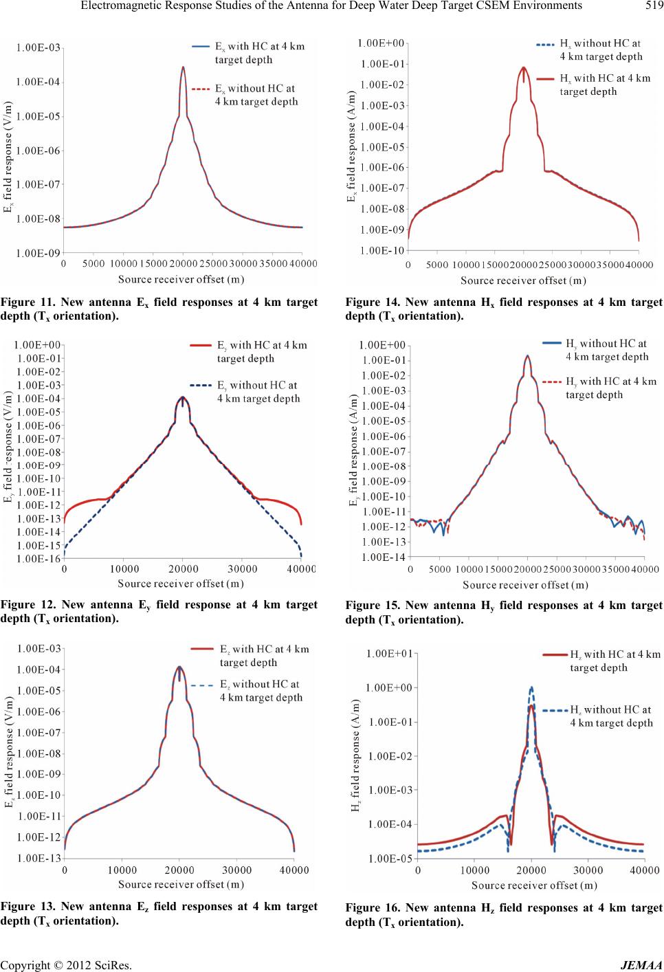

Electromagnetic Response Studies of the Antenna for Deep Water Deep Target CSEM Environments 519
Figure 11. New antenna Ex field responses at 4 km target
depth (Tx orientation).
Figure 12. New antenna Ey field response at 4 km target
depth (Tx orientation).
Figure 13. New antenna Ez field responses at 4 km target
depth (Tx orientation).
Figure 14. New antenna Hx field responses at 4 km target
depth (Tx orientation).
Figure 15. New antenna Hy field responses at 4 km target
depth (Tx orientation).
Figure 16. New antenna Hz field responses at 4 km target
depth (Tx orientation).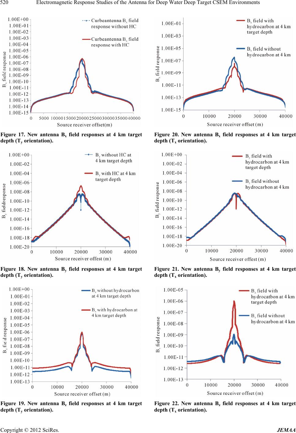

Electromagnetic Response Studies of the Antenna for Deep Water Deep Target CSEM Environments
520
Figure 17. New antenna Bx field responses at 4 km target
depth (Ty orientation).
Figure 18. New antenna By field responses at 4 km target
depth (Ty orientation).
Figure 19. New antenna Bz field responses at 4 km target
depth (Ty orientation).
Figure 20. New antenna Bx field responses at 4 km target
depth (Tx orientation).
Figure 21. New antenna By field responses at 4 km target
depth (Tx orientation).
Figure 22. New antenna Bz field responses at 4 km target
epth (Tx orientation). d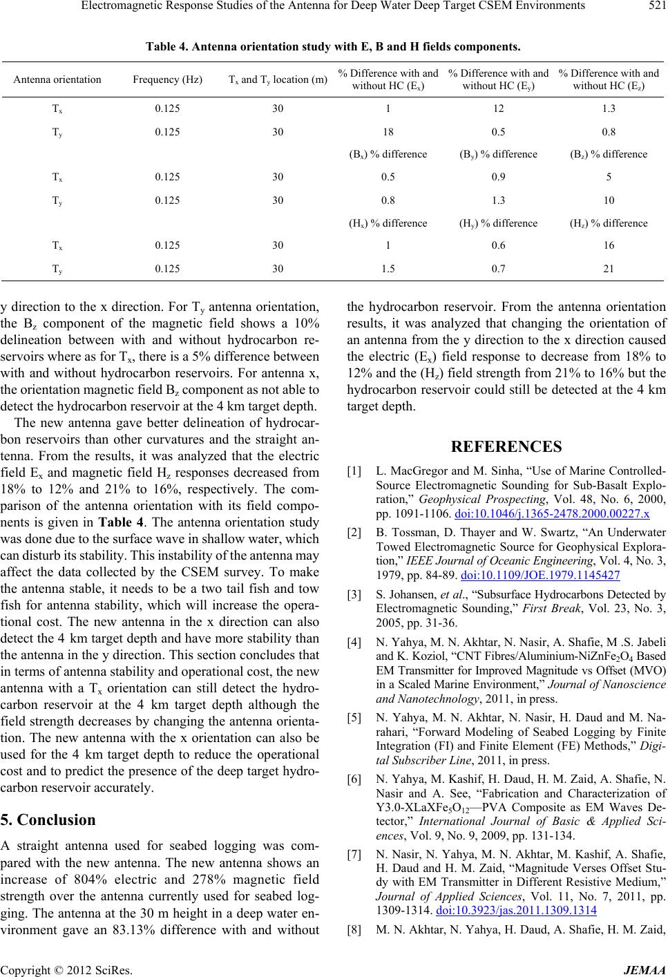

Electromagnetic Response Studies of the Antenna for Deep Water Deep Target CSEM Environments
521
Table 4. Antenna orientation study with E, B and H fields components.
Antenna orientation Frequency (Hz) Tx and Ty location (m)% Difference with and
without HC (Ex)
% Difference with and
without HC (Ey)
% Difference with and
without HC (Ez)
Tx 0.125 30 1 12 1.3
Ty 0.125 30 18 0.5 0.8
(Bx) % difference (By) % difference (Bz) % difference
Tx 0.125 30 0.5 0.9 5
Ty 0.125 30 0.8 1.3 10
(Hx) % difference (Hy) % difference (Hz) % difference
Tx 0.125 30 1 0.6 16
Ty 0.125 30 1.5 0.7 21
y direction to the x direction. For Ty antenna orientation,
the Bz component of the magnetic field shows a 10%
delineation between with and without hydrocarbon re-
servoirs where as for Tx, there is a 5% difference between
with and without hydrocarbon reservoirs. For antenna x,
the orientation magnetic field Bz component as not able to
detect the hydrocarbon reservoir at the 4 km target depth.
The new antenna gave better delineation of hydrocar-
bon reservoirs than other curvatures and the straight an-
tenna. From the results, it was analyzed that the electric
field Ex and magnetic field Hz responses decreased from
18% to 12% and 21% to 16%, respectively. The com-
parison of the antenna orientation with its field compo-
nents is given in Table 4. The antenna orientation study
was done due to the surface wave in shallow water, which
can disturb its stability. This instability of the antenna may
affect the data collected by the CSEM survey. To make
the antenna stable, it needs to be a two tail fish and tow
fish for antenna stability, which will increase the opera-
tional cost. The new antenna in the x direction can also
detect the 4 km target depth and have more stability than
the antenna in the y direction. This section concludes that
in terms of antenna stability and operational cost, the new
antenna with a Tx orientation can still detect the hydro-
carbon reservoir at the 4 km target depth although the
field strength decreases by changing the antenna orienta-
tion. The new antenna with the x orientation can also be
used for the 4 km target depth to reduce the operational
cost and to predict the presence of the deep target hydro-
carbon reservoir accurately.
5. Conclusion
A straight antenna used for seabed logging was com-
pared with the new antenna. The new antenna shows an
increase of 804% electric and 278% magnetic field
strength over the antenna currently used for seabed log-
ging. The antenna at the 30 m height in a deep water en-
vironment gave an 83.13% difference with and without
the hydrocarbon reservoir. From the antenna orientation
results, it was analyzed that changing the orientation of
an antenna from the y direction to the x direction caused
the electric (Ex) field response to decrease from 18% to
12% and the (Hz) field strength from 21% to 16% but the
hydrocarbon reservoir could still be detected at the 4 km
target depth.
REFERENCES
[1] L. MacGregor and M. Sinha, “Use of Marine Controlled-
Source Electromagnetic Sounding for Sub-Basalt Explo-
ration,” Geophysical Prospecting, Vol. 48, No. 6, 2000,
pp. 1091-1106. doi:10.1046/j.1365-2478.2000.00227.x
[2] B. Tossman, D. Thayer and W. Swartz, “An Underwater
Towed Electromagnetic Source for Geophysical Explora-
tion,” IEEE Journal of Oceanic Engineering, Vol. 4, No. 3,
1979, pp. 84-89. doi:10.1109/JOE.1979.1145427
[3] S. Johansen, et al., “Subsurface Hydrocarbons Detected by
Electromagnetic Sounding,” First Break, Vol. 23, No. 3,
2005, pp. 31-36.
[4] N. Yahya, M. N. Akhtar, N. Nasir, A. Shafie, M .S. Jabeli
and K. Koziol, “CNT Fibres/Aluminium-NiZnFe2O4 Based
EM Transmitter for Improved Magnitude vs Offset (MVO)
in a Scaled Marine Environment,” Journal of Nanoscience
and Nanotechnology, 2011, in press.
[5] N. Yahya, M. N. Akhtar, N. Nasir, H. Daud and M. Na-
rahari, “Forward Modeling of Seabed Logging by Finite
Integration (FI) and Finite Element (FE) Methods,” Digi-
tal Subscriber Line, 2011, in press.
[6] N. Yahya, M. Kashif, H. Daud, H. M. Zaid, A. Shafie, N.
Nasir and A. See, “Fabrication and Characterization of
Y3.0-XLaXFe5O12—PVA Composite as EM Waves De-
tector,” International Journal of Basic & Applied Sci-
ences, Vol. 9, No. 9, 2009, pp. 131-134.
[7] N. Nasir, N. Yahya, M. N. Akhtar, M. Kashif, A. Shafie,
H. Daud and H. M. Zaid, “Magnitude Verses Offset Stu-
dy with EM Transmitter in Different Resistive Medium,”
Journal of Applied Sciences, Vol. 11, No. 7, 2011, pp.
1309-1314. doi:10.3923/jas.2011.1309.1314
[8] M. N. Akhtar, N. Yahya, H. Daud, A. Shafie, H. M. Zaid,

Electromagnetic Response Studies of the Antenna for Deep Water Deep Target CSEM Environments
522
M. Kashif and N. Nasir, “Development of EM Wave
Guide Amplifier Potentially Used for Seabed Logging,”
Journal of Applied Sciences, Vol. 11, No. 7, 2011, pp.
1361-1365. doi:10.3923/jas.2011.1361.1365
[9] M. Unsworth, “New Developments in Conventional Hy-
drocarbon Exploration with Electromagnetic Methods,”
CSEG Recorder, Vol. 30, No. 4, 2005, pp. 34-38.
[10] P. Clemmow, “The Theory of Electromagnetic Waves in
a Simple Vanisotropic Medium,” Proceedings of the In-
stitution of Electrical Engineers, Vol. 110, No. 1, 1963,
pp. 101-106. doi:10.1049/piee.1963.0015
[11] F. N. Kong, H. Weterdahl, S. Ellingsrud, T. Eidesmo and
S. Johansen, “A Possible Direct Hydrocarbon Indicator
for Deep Sea Prospects Using EM Energy,” Oil and Gas
Journal, Vol. 100, No. 19, 2002, pp. 30-38.
[12] M. N. Akhtar, N. Yahya, K. Koziol and N. Nasir, “Syn-
thesis and Characterizations of
Ni0.8Zn0.2Fe2O4—MWCNTs Composites for Their Appli-
cation in Sea Bed Logging,” Ceramics International, Vol.
37, No. 8, 2011, pp. 3237-3245.
doi:10.1016/j.ceramint.2011.05.113
[13] M. C. Sinha, P. D. Patel, M. J. Unsworth, T. R. E. Owen
and M. G. R. MacCormack, “An Active Source Electro-
Magnetic Sounding System for Marine Use,” Marine
Geophysical Research, Vol. 12, No. 1-2, 1990, pp. 59-68.
[14] J. Nordskag and L. Amundsen, “Asymptotic Airwave Mo-
deling for Marine Controlled-Source Electromagnetic Sur-
veying,” Geophysics, Vol. 72, No. 6, 2007, pp. F249-F255.
doi:10.1190/1.2786025
[15] Y. Li and K. Key, “2D Marine Controlled Electromag-
netic Modeling: An Adaptive Finite Element Algori-
them,” Geophysics, Vol. 72, No. 2, 2007, pp. 51-62.
doi:10.1190/1.2432262
[16] F. N. Kong, S. E. Johnstad and T. Roesten, “Characte-
ristics of Scattered Fields from Hydrocarbon Layers in
Seabed Logging,” PIERS Online, Vol. 2, No. 6, 2006, pp.
585-588. doi:10.2529/PIERS060821070831
[17] P. D. Young and C. S. Cox, “Electromagnetic Active Source
Sounding Near the East Pacific Rise,” Geophysical Re-
search Letters, Vol. 8, No. 10, 1981, pp. 1043-1046.
doi:10.1029/GL008i010p01043
[18] E. Um and D. Alumbaugh, “On the Physics of the Marine
Controlled-Source Electromagnetic Method,” Geophysics,
Vol. 72, No. 2, 2007, pp. WA13-WA26.
doi:10.1190/1.2432482
[19] S. Ellingsrud, T. Eidesmo, S. Johansen, M. C. Sinha, L.
M. MacGregor and S. Constabl, “The Leading Edge,” So-
ciety of Economic Geologists, Vol. 21, No. 10, 2002, pp.
972-982. doi:10.1190/1.1518433
[20] S. C. Constable, C. S. Cox and A. D. Chave, “Offshore
Electromagnetic Surveying Techniques,” 1986 SEG An-
nual Meeting, 1986.
[21] P. D. Aversana and M. Vivier, “Geophysical Prospecting,
Expanding the Frequency Spectrum in Marine CSEM
Applications,” Geophysical Prospecting, Vol. 57, No. 4,
2008, pp. 573-590.
[22] F. Maao and F. A. Roth, “Improving Seabed Logging Sen-
sitivity in Shallow Water through Up-Down Separation,”
EGM 2007 International Workshop, Trondhiem, 2007.
[23] J. A. Kong, “Electromagnetic Wave Theory,” John Wiley
and Sons, New York, 1986.
[24] A. Shaw, A. I. Al-Shamma’a, S. R. Wylie and D. Toal,
“Experimental Investigations of Electromagnetic Wave
Propagation in Seawater,” Proceedings of the 36th Euro-
pean Microwave Conference, Manchester, 10-15 Septem-
ber 2006, pp. 572-575.
[25] Sodal, “Transmitting Antenna,” US Patent No. 0202697,
2006.
[26] H. Daud, N. Yahya and R. Harun, “Wireless Control Me-
chanisim for EM Source and Receiver Positioning for Off-
shore Applications,” Journal of Applied Science, Vol. 11,
No. 7, 2011, pp. 1812-5654.
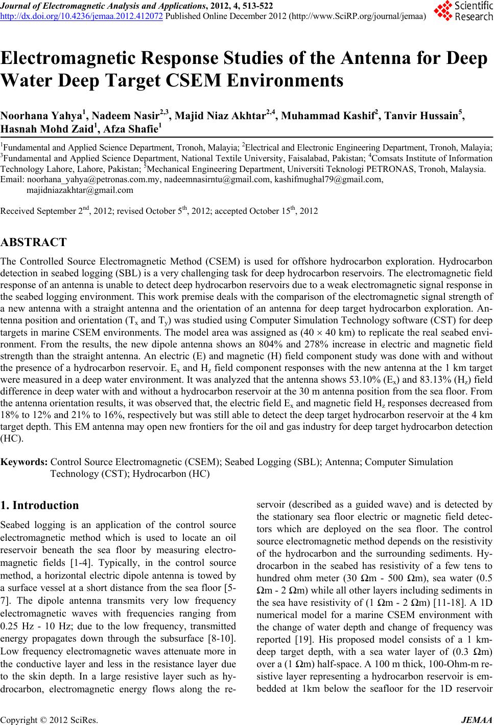