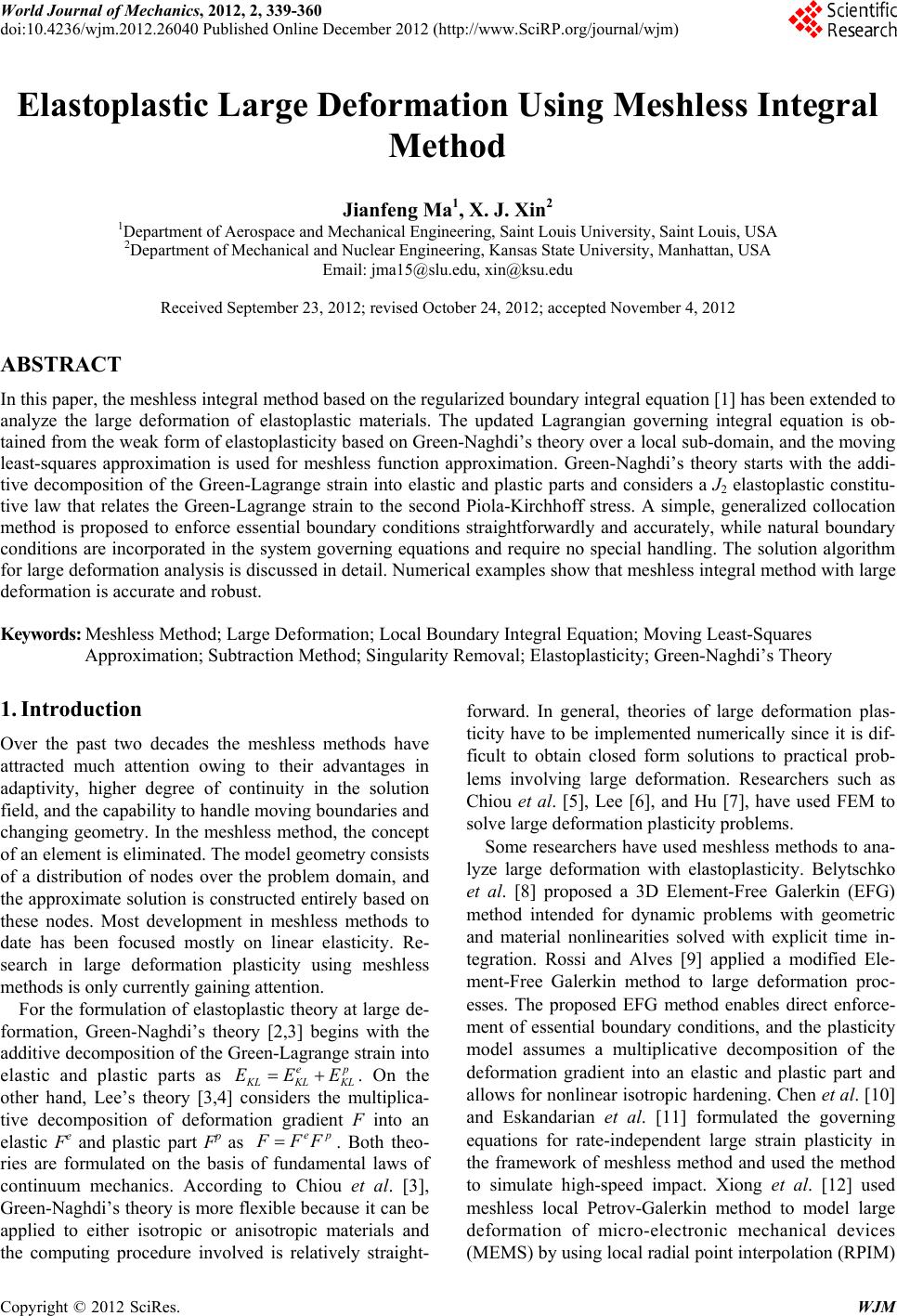
 World Journal of Mechanics, 2012, 2, 339-360 doi:10.4236/wjm.2012.26040 Published Online December 2012 (http://www.SciRP.org/journal/wjm) Copyright © 2012 SciRes. WJM Elastoplastic Large Deformation Using Meshless Integral Method Jianfeng Ma1, X. J. Xin2 1Department of Aerospace and Mechanical Engineering, Saint Louis University, Saint Louis, USA 2Department of Mechanical and Nuclear Engineering, Kansas State University, Manhattan, USA Email: jma15@slu.edu, xin@ksu.edu Received September 23, 2012; revised October 24, 2012; accepted November 4, 2012 ABSTRACT In this paper, the meshless integral method based on the regularized boundary integral equation [1] has been extended to analyze the large deformation of elastoplastic materials. The updated Lagrangian governing integral equation is ob- tained from the weak form of elastoplasticity based on Green-Naghdi’s theory over a local sub-domain, and the moving least-squares approximation is used for meshless function approximation. Green-Naghdi’s theory starts with the addi- tive decomposition of the Green-Lagrange strain into elastic and plastic parts and considers a J2 elastoplastic constitu- tive law that relates the Green-Lagrange strain to the second Piola-Kirchhoff stress. A simple, generalized collocation method is proposed to enforce essential boundary conditions straightforwardly and accurately, while natural boundary conditions are incorporated in the system governing equations and require no special handling. The solution algorithm for large deformation analysis is discussed in detail. Numerical examples show that meshless integral method with large deformation is accurate and robust. Keywords: Meshless Method; Large Deformation; Local Boundary Integral Equation; Moving Least-Squares Approximation; Subtraction Method; Singularity Removal; Elastoplasticity; Green-Naghdi’s Theory 1. Introduction Over the past two decades the meshless methods have attracted much attention owing to their advantages in adaptivity, higher degree of continuity in the solution field, and the capability to handle moving boundaries and changing geometry. In the meshless method, the concept of an element is eliminated. The model geometry consists of a distribution of nodes over the problem domain, and the approximate solution is constructed entirely based on these nodes. Most development in meshless methods to date has been focused mostly on linear elasticity. Re- search in large deformation plasticity using meshless methods is only currently gaining attention. For the formulation of elastoplastic theory at large de- formation, Green-Naghdi’s theory [2,3] begins with the additive decomposition of the Green-Lagrange strain into elastic and plastic parts as ep LKLKL EEE . On the other hand, Lee’s theory [3,4] considers the multiplica- tive decomposition of deformation gradient F into an elastic Fe and plastic part Fp as ep FF. Both theo- ries are formulated on the basis of fundamental laws of continuum mechanics. According to Chiou et al. [3], Green-Naghdi’s theory is more flexible because it can be applied to either isotropic or anisotropic materials and the computing procedure involved is relatively straight- forward. In general, theories of large deformation plas- ticity have to be implemented numerically since it is dif- ficult to obtain closed form solutions to practical prob- lems involving large deformation. Researchers such as Chiou et al. [5], Lee [6], and Hu [7], have used FEM to solve large deformation plasticity problems. Some researchers have used meshless methods to ana- lyze large deformation with elastoplasticity. Belytschko et al. [8] proposed a 3D Element-Free Galerkin (EFG) method intended for dynamic problems with geometric and material nonlinearities solved with explicit time in- tegration. Rossi and Alves [9] applied a modified Ele- ment-Free Galerkin method to large deformation proc- esses. The proposed EFG method enables direct enforce- ment of essential boundary conditions, and the plasticity model assumes a multiplicative decomposition of the deformation gradient into an elastic and plastic part and allows for nonlinear isotropic hardening. Chen et al. [10] and Eskandarian et al. [11] formulated the governing equations for rate-independent large strain plasticity in the framework of meshless method and used the method to simulate high-speed impact. Xiong et al. [12] used meshless local Petrov-Galerkin method to model large deformation of micro-electronic mechanical devices (MEMS) by using local radial point interpolation (RPIM) 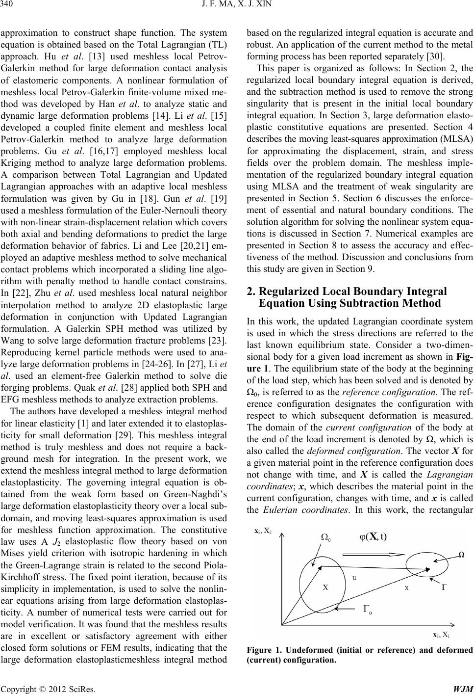 J. F. MA, X. J. XIN Copyright © 2012 SciRes. WJM 340 approximation to construct shape function. The system equation is obtained based on the Total Lagrangian (TL) approach. Hu et al. [13] used meshless local Petrov- Galerkin method for large deformation contact analysis of elastomeric components. A nonlinear formulation of meshless local Petrov-Galerkin finite-volume mixed me- thod was developed by Han et al. to analyze static and dynamic large deformation problems [14]. Li et al. [15] developed a coupled finite element and meshless local Petrov-Galerkin method to analyze large deformation problems. Gu et al. [16,17] employed meshless local Kriging method to analyze large deformation problems. A comparison between Total Lagrangian and Updated Lagrangian approaches with an adaptive local meshless formulation was given by Gu in [18]. Gun et al. [19] used a meshless formulation of the Euler-Nernouli theory with non-linear strain-displacement relation which covers both axial and bending deformations to predict the large deformation behavior of fabrics. Li and Lee [20,21] em- ployed an adaptive meshless method to solve mechanical contact problems which incorporated a sliding line algo- rithm with penalty method to handle contact constrains. In [22], Zhu et al. used meshless local natural neighbor interpolation method to analyze 2D elastoplastic large deformation in conjunction with Updated Lagrangian formulation. A Galerkin SPH method was utilized by Wang to solve large deformation fracture problems [23]. Reproducing kernel particle methods were used to ana- lyze large deformation problems in [24-26]. In [27], Li et al. used an element-free Galerkin method to solve die forging problems. Quak et al. [28] applied both SPH and EFG meshless methods to analyze extraction problems. The authors have developed a meshless integral method for linear elasticity [1] and later extended it to elastoplas- ticity for small deformation [29]. This meshless integral method is truly meshless and does not require a back- ground mesh for integration. In the present work, we extend the meshless integral method to large deformation elastoplasticity. The governing integral equation is ob- tained from the weak form based on Green-Naghdi’s large deformation elastoplasticity theory over a local sub- domain, and moving least-squares approximation is used for meshless function approximation. The constitutive law uses A J2 elastoplastic flow theory based on von Mises yield criterion with isotropic hardening in which the Green-Lagrange strain is related to the second Piola- Kirchhoff stress. The fixed point iteration, because of its simplicity in implementation, is used to solve the nonlin- ear equations arising from large deformation elastoplas- ticity. A number of numerical tests were carried out for model verification. It was found that the meshless results are in excellent or satisfactory agreement with either closed form solutions or FEM results, indicating that the large deformation elastoplasticmeshless integral method based on the regularized integral equation is accurate and robust. An application of the current method to the metal forming process has been reported separately [30]. This paper is organized as follows: In Section 2, the regularized local boundary integral equation is derived, and the subtraction method is used to remove the strong singularity that is present in the initial local boundary integral equation. In Section 3, large deformation elasto- plastic constitutive equations are presented. Section 4 describes the moving least-squares approximation (MLSA) for approximating the displacement, strain, and stress fields over the problem domain. The meshless imple- mentation of the regularized boundary integral equation using MLSA and the treatment of weak singularity are presented in Section 5. Section 6 discusses the enforce- ment of essential and natural boundary conditions. The solution algorithm for solving the nonlinear system equa- tions is discussed in Section 7. Numerical examples are presented in Section 8 to assess the accuracy and effec- tiveness of the method. Discussion and conclusions from this study are given in Section 9. 2. Regularized Local Boundary Integral Equation Using Subtraction Method In this work, the updated Lagrangian coordinate system is used in which the stress directions are referred to the last known equilibrium state. Consider a two-dimen- sional body for a given load increment as shown in Fig- ure 1. The equilibrium state of the body at the beginning of the load step, which has been solved and is denoted by Ω0, is referred to as the reference configuration. The ref- erence configuration designates the configuration with respect to which subsequent deformation is measured. The domain of the current configuration of the body at the end of the load increment is denoted by Ω, which is also called the deformed configuration. The vector X for a given material point in the reference configuration does not change with time, and X is called the Lagrangian coordinates; x, which describes the material point in the current configuration, changes with time, and x is called the Eulerian coordinates. In this work, the rectangular Figure 1. Undeformed (initial or reference) and deformed (current) configuration.  J. F. MA, X. J. XIN Copyright © 2012 SciRes. WJM 341 Eulerian coordinates, xk (k = 1, 2), and Lagrangian coor- dinates, XK (K = 1, 2), are employed. We use upper case letter and upper case subscript to indicate that the vari- able of interest refers to the reference state, and use lower case letter and lower case subscript to indicate that the variable of interest refers to the current state. Within the updated Lagrangian framework, the following proce- dures are implied: 1) During each load increment, all field variables are defined with respect to the state at the start of this load increment (reference configuration); 2) At the end of this load increment, field variables are up- dated with respect to the state at the end of this load in- crement (current configuration), and the current configu- ration will be the reference configuration for the next load increment. In large deformation problems, various stress measures can be defined. The most commonly used stresses are: 1) Cauchy stress (true stress) tensor σ which expresses the stress relative to the current configuration; 2) First Piola- Kirchhoff stress (nominal stress) tensor P which relates forces in the current configuration with areas in the reference configuration; 3) Second Piola-Kirchhoff stress tensor T which relates forces in the reference configuration to areas in the reference configuration, where the force in the reference configuration is obtained via a mapping that preserves the relative relationship between the force direction and the area normal in the current configuration. The relationships between these stresses are 11T ,,JJ PFσTFσF where F is the deformation gradient and defined as x Y yy Y F, and J is the determinant of F. The second Piola-Kirchhoff stress tensor is symmetric, and in the current work is linked to the Green-Lagrange strain in the elastoplastic constitutive law. For a large deformation elastoplastic body represented by a reference domain Ω0 with boundary Γ0, the govern- ing elastoplasticity equations are as follows: ,0 ,,,, 0 0 1, 2 Ω IJ JI IJI JJ IKIK J ecor IJIJKL KLIJ f E uuuu dTCdEdT XX XX XX X XXX (1) where τ (bold face denotes vectors or tensors) is the stress measure defined by r IJ rIrJ rILJ L GGT , TLJ is the second Piola-Kirchhoff stress, G is the trans- formation tensor between the reference configuration and the current configuration, r is the deformation gra- dient, E is the Green strain tensor associated with the displacement u, ρ0 is the mass density in the reference configuration Ω0, fI is the body force per unit mass, e JKL C is the linear elastic stiffness matrix, and cor J dT is the stress correction term because of nonlinearities in either geometry or material. An index I following a comma designates partial differentiation with respect to XI, and repeated indices indicate summation over the dimensionality of the problem. The essential and the natural boundary conditions on the boundary Γ are re- spectively: on Iu uu (2) on IJ JIt TnT (3) here, u represents the prescribed displacement on u , T represents the prescribed traction on t ; n is the outward unit normal to the boundary; tu and tu . The weak form of (1) over a local sub-domain 00 a in the reference state is: 0 ,0 0 ,d 0 a a IJ JII fg XXXYX (4) where the notation in this paper is used to denote a node (e.g., a indicates node a, b indicates node b, etc.) in order to reserve the usual subscripts, I, J, etc., for denoting degree of freedom (DOF) components, 00 a is a spherical (circular in 2D) sub-domain related to node a, a Y is the position vector of node a which is also called a source point, X is the integration or field point which may or may not coincide with a node, and is the test function. In the following, the func- tional dependence on X, i.e. “(X)”, will be dropped for brevity when no ambiguity is caused. In this work, fol- lowing [31], we use a special test function defined by ,, aaa IJIJ gue XYXYY (5) where e represents the J-th component of a unit force vector, I u is the special test function, given by [31]: 2 2 2 22 , 1 8π1 54 43ln 1 23 4 1 a IJ aa J aa ss aa a IJ aa s u rvr v hh rr r hr XY (6)  J. F. MA, X. J. XIN Copyright © 2012 SciRes. WJM 342 where a r is the distance from a Y to X; aa II rXY; a n is the outward unit normal to the boundary 0 a at X; a h is the radius of the local sub-domain; and EE for plane strain, or 1 and 2 1EE for plane stress; E is the Young’s modulus, is the Poisson’s ratio, and 21E is the shear modulus. Note that the special test function is defined in the reference state. The associated traction, for linear elastic behavior, is 2 32 2 , 11 12 4π134 12 2 3 34 a IJ aa a KK J aa a s aa a aa aa IJ IJ JI aa a aa aa IJ JI a s t rn rv vrn vh rr rv rnrn nr r rnrn vh XY (7) The special test function J u has the property that it vanishes on the boundary of a spherical 0 a . With J u as the test function, application of integration by parts to (4) twice leads to: 0 0 0 0 0 0 0 *0 , ,,, 0 , , ,d ,d ,d ,d ,d ,d ,d a a a a a a a a I a IJ J a IJ J acor r IJ KLKrJ L ae IJKRJR LLKMNMN a IJLKJ LK a IJLKJLJ LK u uT tu x uT X uuCu uTun uT un XYX X XYX X XYX X XY XX XY X XYXX X YX XX 0 0 ,d0 a a IJ J uf XYX X (8) where 0 a is the boundary of 0 a , 0 T is the J-th component of the traction at the reference state, u is the displacement increment from the reference state to the current state, 0 K T is the second Piola-Kirchhoff stress at the reference state, K T is the second Piola- Kirchhoff stress increment from the reference state to the current state, and ,a XY is the Dirac delta function. Equation (8) in its current form cannot be used directly in numerical calculation because when a Y is a boundary node, the equation contains strong singularity (1/r type in line integral) in the traction term J t . For the local inte- gral equation approach to be a valid numerical method, the strong singularity must be handled appropriately. The subtraction technique is employed in the present study to remove the strong singularity; the technique for small deformation has been presented in 4[1]. For simplic- ity in implementation, the local sub-domain is always chosen, in the reference state, as a sphere or part of a sphere centered on a node. If node a Y is an interior node, a h is selected such that 0 a stays fully inside 0 . If a Y is a boundary node, then 0 a is the in- tersection of 0 and a sphere a of radius a h, centered at the boundary node, and the boundary 0 a is the union of the part of a inside 0 , denoted by a C, and the part of 0 inside a , denoted by Γa, as illustrated in Figure 2. A further modifica- tion is the exclusion of a tiny sphere of radius Δ (which later tends to zero) centered on a Y whose boundary is denoted by a C. Figure 3 shows sche- matically this modification. For interior nodes, Γa is empty, and a C is a full circle. With the above notations, the boundary 0 a can be decomposed into the following sections: 0Γ aaaa CC (9) aaa ut (10) where a u is the section of a where the displace- ment is prescribed, and a t the section where the trac- tion is prescribed. Using subtraction method, we obtain, in the limit of 0 , the following: Figure 2. Schematic diagram showing the sub-domain for an interior or a boundary node a Y. 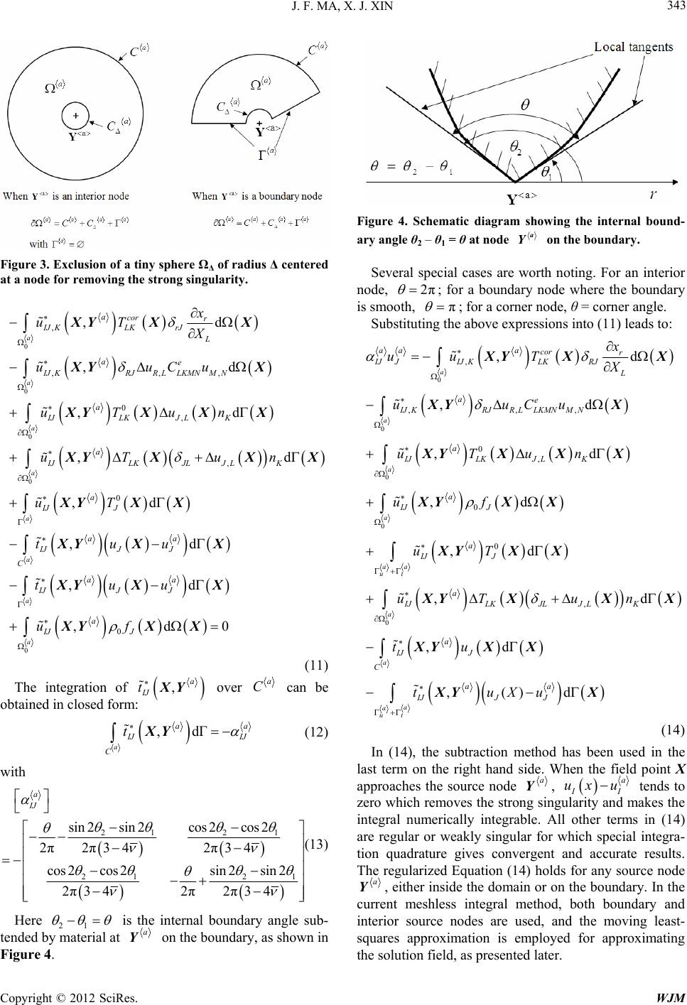 J. F. MA, X. J. XIN Copyright © 2012 SciRes. WJM 343 Figure 3. Exclusion of a tiny sphere ΩΔ of radius Δ centered at a node for removing the strong singularity. 0 0 0 0 , ,,, 0 , , 0 ,d ,d ,d ,d ,d ,d ,d a a a a a a acor r IJ KLKrJ L ae IJKRJR LLKMNMN a IJLKJ LK a IJLKJLJ LK a IJ J aa IJJ J C aa IJJ J x uT X uuCu uTun uT un uT tuu tuu XY XX XY X XYXXX YX XX XYX X XY XX XY X 0 0 ,d0 a a a IJ J uf X XYX X (11) The integration of ,a IJ t XY over a C can be obtained in closed form: ,dΓ a aa JIJ C t XY (12) with 212 1 21 21 sin 2sin 2cos2cos 2 2π2π34 2π34 cos 2cos 2sin2sin2 2π34 2π2π34 a IJ (13) Here 21 is the internal boundary angle sub- tended by material at a Y on the boundary, as shown in Figure 4. Figure 4. Schematic diagram showing the internal bound- ary angle θ2 – θ1 = θ at node a Y on the boundary. Several special cases are worth noting. For an interior node, 2π ; for a boundary node where the boundary is smooth, π ; for a corner node, θ = corner angle. Substituting the above expressions into (11) leads to: 0 0 0 0 0 , ,,, 0 , 0 0 , ,d ,d ,d ,d ,d ,d a a a a a a ut a aaa cor r IJJIJ KLKRJ L ae IJKRJR LLKMNMN a IJLKJ LK a IJ J a IJ J a IJLKJLJ LK IJ x uuT X uuCu uTun uf uT uT un t YX X XY X XYXXX XYX X XYX X YX XX X ,d ,()d a a a ut a J C aa IJJ J u tuXu YXX XY X (14) In (14), the subtraction method has been used in the last term on the right hand side. When the field point X approaches the source node a Y, a I ux u tends to zero which removes the strong singularity and makes the integral numerically integrable. All other terms in (14) are regular or weakly singular for which special integra- tion quadrature gives convergent and accurate results. The regularized Equation (14) holds for any source node a Y, either inside the domain or on the boundary. In the current meshless integral method, both boundary and interior source nodes are used, and the moving least- squares approximation is employed for approximating the solution field, as presented later. 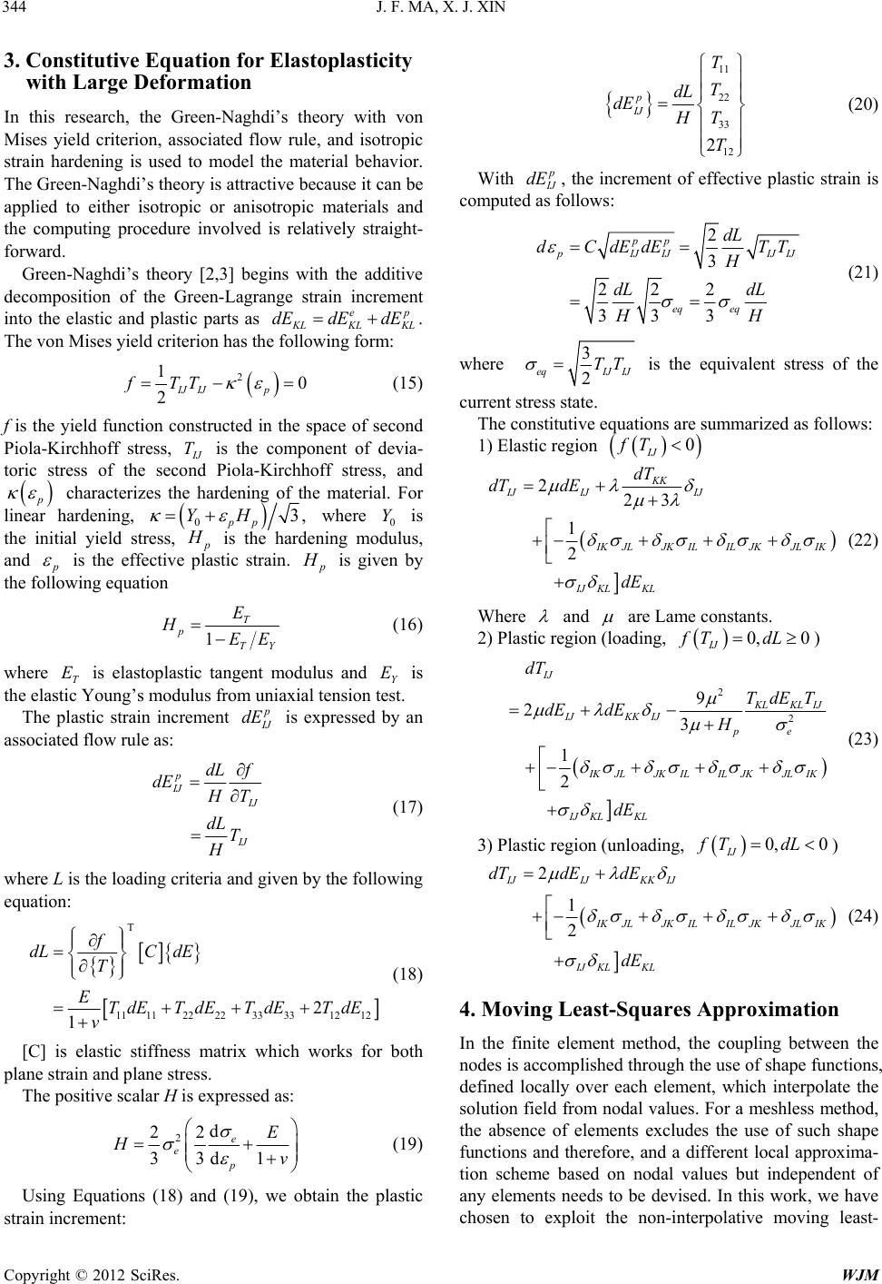 J. F. MA, X. J. XIN Copyright © 2012 SciRes. WJM 344 3. Constitutive Equation for Elastoplasticity with Large Deformation In this research, the Green-Naghdi’s theory with von Mises yield criterion, associated flow rule, and isotropic strain hardening is used to model the material behavior. The Green-Naghdi’s theory is attractive because it can be applied to either isotropic or anisotropic materials and the computing procedure involved is relatively straight- forward. Green-Naghdi’s theory [2,3] begins with the additive decomposition of the Green-Lagrange strain increment into the elastic and plastic parts as ep LKLKL dEdE dE . The von Mises yield criterion has the following form: 2 10 2IJ IJp fTT (15) f is the yield function constructed in the space of second Piola-Kirchhoff stress, J T is the component of devia- toric stress of the second Piola-Kirchhoff stress, and characterizes the hardening of the material. For linear hardening, 03, pp YH where 0 Y is the initial yield stress, is the hardening modulus, and is the effective plastic strain. is given by the following equation 1 T p TY E HEE (16) where T E is elastoplastic tangent modulus and Y E is the elastic Young’s modulus from uniaxial tension test. The plastic strain increment J dE is expressed by an associated flow rule as: p IJ J IJ dL f dE T dL T H (17) where L is the loading criteria and given by the following equation: T 11 11222233 331212 2 1 f dLC dE T ETdE TdETdETdE v (18) [C] is elastic stiffness matrix which works for both plane strain and plane stress. The positive scalar H is expressed as: 2d 22 33d1 e e p E Hv (19) Using Equations (18) and (19), we obtain the plastic strain increment: 11 22 33 12 2 p IJ T T dL dE T H T (20) With J dE , the increment of effective plastic strain is computed as follows: 2 3 22 2 33 3 pp IJIJIJ IJ eq eq dL dCdEdET T H dL dL HH (21) where 3 2 eqIJ IJ TT is the equivalent stress of the current stress state. The constitutive equations are summarized as follows: 1) Elastic region 0 IJ fT 223 1 2 KK IJ IJIJ KJL JKIL ILJKJLIK IJ KLKL dT dT dE dE (22) Where and are Lame constants. 2) Plastic region (loading, 0, 0 IJ fT dL ) 2 2 9 23 1 2 IJ LKLIJ IJKK IJ pe KJL JKIL ILJKJLIK IJ KLKL dT TdET dE dEH dE (23) 3) Plastic region (unloading, 0, 0 IJ fT dL ) 2 1 2 IJIJKK IJ KJL JKIL ILJKJLIK IJ KLKL dTdE dE dE (24) 4. Moving Least-Squares Approximation In the finite element method, the coupling between the nodes is accomplished through the use of shape functions, defined locally over each element, which interpolate the solution field from nodal values. For a meshless method, the absence of elements excludes the use of such shape functions and therefore, and a different local approxima- tion scheme based on nodal values but independent of any elements needs to be devised. In this work, we have chosen to exploit the non-interpolative moving least- 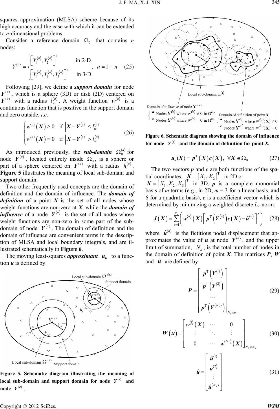 J. F. MA, X. J. XIN Copyright © 2012 SciRes. WJM 345 squares approximation (MLSA) scheme because of its high accuracy and the ease with which it can be extended to n-dimensional problems. Consider a reference domain 0 that contains n nodes: T 12 T 123 , in 2-D , 1 ,, in 3-D aa a aaa YY Yan YYY (25) Following [29], we define a support domain for node a Y, which is a sphere (3D) or disk (2D) centered on a Y with a radius a w l. A weight function a w is a continuous function that is positive in the support domain and zero outside, i.e. a a 0if 0if aa w aa w wl wl XXY XXY (26) As introduced previously, the sub-d oma in 0 a for node a Y, located entirely inside 0 , is a sphere or part of a sphere centered on a Y with a radius a h. Figure 5 illustrates the meaning of local sub-domain and support domain. Two other frequently used concepts are the domain of definition and the domain of influence. The domain of definition of a point X is the set of all nodes whose weight functions are non-zero at X, while the domain of influence of a node a Y is the set of all nodes whose weight functions are non-zero in some part of the sub- domain of node a Y. The domain of definition and the domain of influence are convenient terms in the descrip- tion of MLSA and local boundary integrals, and are il- lustrated schematically in Figure 6. The moving least-squares approximant h u to a func- tion u is defined by: Figure 5. Schematic diagram illustrating the meaning of local sub-domain and support domain for node a Y and node b Y. Figure 6. Schematic diagram showing the domain of influence for node a Y and the domain of definition for point X. T 0 (), h uXp XcXX (27) The two vectors p and c are both functions of the spa- tial coordinates: T 12 ,XXX in 2D or T 123 ,,XXXX in 3D. p is a complete monomial basis of m terms (e.g., in 2D, m = 3 for a linear basis, and 6 for a quadratic basis), c is a coefficient vector which is determined by minimizing a weighted discrete L2-norm: 2 T 1 ˆ x N aaa a w JXXp YcXu (28) where ˆa u is the fictitious nodal displacement that ap- proximates the value of u at node a Y, and the upper limit of summation, N, is the total number of nodes in the domain of definition of point X. The matrices P, W and ˆ u are defined by 1 T 2 T Tx x N Nm pY pY P pY (29) 10 0x xx N NN w w X Wx X (30) 1 2 ˆ ˆ ˆ ˆx N u u u u (31) 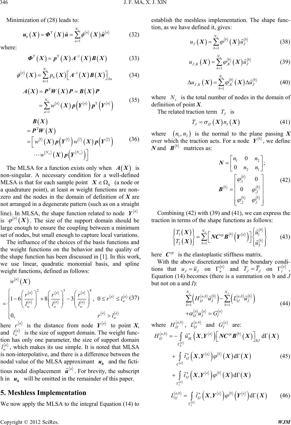 J. F. MA, X. J. XIN Copyright © 2012 SciRes. WJM 346 Minimization of (28) leads to: T 1 ˆˆ x N aa h a uX Φ uXu (32) where: TT1 Φ pXA XBX (33) 1 1 x N a bba b p XXAXBX (34) T T 1 x N aaa a w AXPWX PBX P XpYp Y (35) T 112 2 xx NN ww w BX PW X XpYXpY XpY (36) The MLSA for a function exists only when AX is non-singular. A necessary condition for a well-defined MLSA is that for each sample point 0 X (a node or a quadrature point), at least m weight functions are non- zero and the nodes in the domain of definition of X are not arranged in a degenerate pattern (such as on a straight line). In MLSA, the shape function related to node a Y is a . The size of the support domain should be large enough to ensure the coupling between a minimum set of nodes, but small enough to capture local variations. The influence of the choices of the basis functions and the weight functions on the behavior and the quality of the shape function has been discussed in [1]. In this work, we use linear, quadratic monomial basis, and spline weight functions, defined as follows: 234 1683,0 0, a aaa aa w aaa www aa w w rrrrl lll rl X (37) here a r is the distance from node a Y to point X, and a w l is the size of support domain. The weight func- tion has only one parameter, the size of support domain a w l, which makes its use simple. It is noted that MLSA is non-interpolative, and there is a difference between the nodal value of the MLSA approximant h u and the ficti- tious nodal displacement ˆa u. For brevity, the subscript h in h u will be omitted in the remainder of this paper. 5. Meshless Implementation We now apply the MLSA to the integral Equation (14) to establish the meshless implementation. The shape func- tion, as we have defined it, gives: 1 ˆ x N bb J b uu XX (38) ,, 1 ˆ x N bb KKJ b uu XX (39) ,, 1 ˆ x N bb KKJ b uu XX (40) where N is the total number of nodes in the domain of definition of point X. The related traction term T is JIJ I Tn X (41) where 12 ,nn is the normal to the plane passing X over which the traction acts. For a node b Y, we define N and b matrices as: 12 21 ,1 ,2 ,2 ,1 0; 0 0 0 b bb bb nn nn N B (42) Combining (42) with (39) and (41), we can express the traction in terms of the shape functions as follows: 11 1 22 ˆ ˆ xb N ba ep b b Tu Tu XNC BY X (43) here ep C is the elastoplastic stiffness matrix. With the above discretization and the boundary condi- tions that J uu on a u and J TT on a t , Equation (14) becomes (there is a summation on b and J but not on a and I): ,, 11 ˆˆ yy NN ab babb IJJIJ J bb aa a IJ JI uLu uG (44) where ,ab IJ H, ,ab IJ L and a G are: ,,dΓ ,dΓ ,dΓ a u a a t aba b ep IJ IKKJ ab IJ C ab IJ Hu t t YNCBX X XYXX XYXX (45) ,,dΓ a t aba ba IJ IJ Lt YYX (46)  J. F. MA, X. J. XIN Copyright © 2012 SciRes. WJM 347 0 0 0 0 0 0 ,, ,,, 0 , , ,d ,d , d ,d ,d ,d , a a t a a a a aa IJIJ a IJ J acor IJKLKRJRLRL ae IJKRJR LLKMNMN a IJLKJ LK a IJLKJLJ LK a IJ J Gbu uT uT u uuCu uTun uT un tu XXY X XYX X XY XX XY X XYXX X YX XX XY X d a u a J u YX (47) and the upper limit of summation, y N, is the total num- ber of nodes in the domain of influence of node a Y. The third to sixth terms of Equation (47) are the nonlin- ear terms because of the large deformation and elasto- plasticity. In all numerical examples tested in this work, the body force term is zero. Owing to the subtraction technique, the singularity in the third integral on the right hand side of (45) as X ap- proaches a Y is cancelled by the term in (46), and similarly the seventh integral on the right hand side of (47) is also regularized. Even though the subtraction technique removes the strong singularity, the integrands in the first integral on the right hand side of (45) and the second integral on the right hand side of (47) still contain the weakly singular ln (r) term. The logarithmic singular- ity is integrable, but the accuracy of ordinary Legendre- Gauss integration is poor. We found that the special inte- gration scheme for the logarithmic singularity [22], which is reproduced in Table 1 for completeness, achieves ex- cellent numerical accuracy [1]. The remaining integrals of Equation (45) and Equation (47) are regular for which standard quadrature can be used with good accuracy. In our numerical examples, the numbers of integration points were as follows: 8 integration points for any inte- gral along a straight line, and 8 × 8 integration points for any integral over a sub-domain. For regularized integrals, the usual Legendre-Gauss integration was used. For inte- grals containing logarithmic singularity, the special inte- gration of 8 integration points [32] as listed in Table 1 was used. 6. Enforcement of Boundary Conditions Appropriate boundary conditions need to be enforced in order to solve the simultaneous Equations (44). In mesh- Table 1. Special numerical integration for functions con- taining logarithmic singularity (8 integration points). 1 1 0 1 ln d N ii i rrwfr r Abscissas (ri) Weights (wi) 0.0133 2024 4160 8925 0.1644 1660 4728 0030 0.0797 5042 9013 8949 0.2375 2561 0023 3060 0.1978 7102 9326 1880 0.2268 4198 4431 9190 0.3541 5399 4351 9090 0.1757 5407 9006 0700 0.5294 5857 5234 9170 0.1129 2403 0246 7590 0.7018 1452 9939 1000 0.0578 7221 0717 7821 0.8493 7932 0441 1070 0.0209 7907 3742 1330 0.9533 2645 0056 3600 0.0036 8640 7104 0276 less methods, enforcing the essential (Dirichlet) bound- ary conditions is not as easy as in the finite element method. Because MLSA is non-interpolative, the essen- tial boundary condition cannot be accurately enforced by prescribing values for the fictitious nodal displacements (i.e., ˆaa I uu). A number of techniques for enforcing essential boundary conditions have been developed, in- cluding the collocation methods [33], Lagrange multi- plier method [34], penalty method [35,36], Nitsche’s method [37], coupled meshless-finite element method [38], and other methods [39-43]. The advantages and disadvantages of a variety of methods for enforcing es- sential boundary conditions have been discussed briefly in [1]. A number of collocation methods have been developed. The direct collocation method [33] used the condition ˆaa I uu (48) to replace the row of the discretized weak form equation corresponding to the degree of freedom with prescribed displacement a u. This is actually inconsistent with the assumption of MLSA since the fictitious nodal displace- ment ˆa u is generally not equal to the approximated displacement value. A generalized collocation method uses 1 ˆ n ababa II b uYuu (49) as the collocation condition which was shown to yield more accurate results [44]. Wagner and Liu [45] devel- oped a corrected collocation method which restores the consistency of the weak form and enhances convergence. Wu and Plesha [46] proposed a boundary flux colloca- tion method to enforce the boundary conditions exactly.  J. F. MA, X. J. XIN Copyright © 2012 SciRes. WJM 348 Generally, there are two types of discretization in meshless methods: 1) Galerkin based method over the global domain, which is used in EFG [33,42,47,48], clouds [41], RKPM [49-52]; and 2) loca l weak for m over multiple local domains, which is employed in [31,53-55]. For Galerkin based method over the global domain, the n system equations are obtained by applying the weak form over the global domain once, hence all equations must hold simultaneously in order to maintain consistency of the weak form. Replacing a row in the matrix equation by (49), which contains a linear combination of DOFs rather than dictating the single value of a constrained DOF, sacrifices the consistency of the weak form and compromises the solution accuracy. For local weak form over multiple local domains, each equation is obtained by applying the weak form over a particular local domain, and the weak form needs to be applied n times for a problem with n DOFs. Conse- quently, the generalized collocation method with (49) can be directly used to enforce essential boundary condi- tions. Because each system equation is independent of the rest, replacing the equation corresponding to a con- strained DOF by (49) will not cause any inconsistency in the weak form. As the current meshless integral method uses local weak form over multiple sub-domains, the generalized collocation method (49) is applicable. For a DOF with essential boundary condition, we simply use the condi- tion I uu rather than applying the integral Equation (14). In numerical implementation, this means replacing the governing equation corresponding to the prescribed DOF with generalized collocation condition (49). Note that the governing Equation (14) holds for interior nodes as well as boundary (including corner) nodes, therefore Equation (49) is applied to nodes on smooth boundaries as well as at corners. Our numerical tests show that the generalized collocation method (49) for enforcing essen- tial boundary conditions works well for the meshless integral method. For the natural boundary condition I tt, no special treatment is needed. The prescribed traction is directly used in the second integral in Equation (47). Although theoretically essential boundary conditions can be converted into the equivalent natural boundary conditions and the solution remains unchanged, we ob- served that the meshless method is always more accurate when essential boundary conditions are used. After the boundary conditions are enforced, the gov- erning equations can be written as , 1 ˆ y N ab ba IJ JI b uR (50) where ,, ,when is unconstrained when ababa ba IJIJ IJ a ab I IJ ba IJ aa II HL u K uu Y Y (51) when is unconstrained when aa aII Iaaa III Gu R uuu (52) and the upper limit of summation, y N, is the total num- ber of nodes in the domain of influence of node a Y. Detailed expressions of various terms are given in Equa- tions (45) to (47). 7. Solution Algorithm for Elastoplasticity with Large Deformation In this work, we will use the fixed point iteration to solve the governing equations which has the following advan- tages: the derivative of the stiffness matrix is not needed, and the implementation is relatively easy. With this algo- rithm, for each load increment, the stiffness matrix is computed only once in the first iteration. The material considered in this study is rate inde- pendent, and therefore the actual loading rate has no ef- fect on the solution. It is, however, convenient to intro- duce a time parameter to describe the loading history. A piecewise linear function is used in the program to de- scribe the history of applied loads and is implemented in a table form in the input data. Each linear segment is referred to as a load step. For a loading history with N load steps, the corresponding data block takes the fol- lowing form: 00 11 22 , , , , N N tP tP tP tP where n indicates the number of load steps. 01 ,,, tt t are the times, while 01 ,, , PP P are the corresponding load levels. Both 0 t and 0 P are set to zero if the initial state is load free. Since the elastoplastic integral equations are strongly nonlinear, loads have to be applied in small increments, and iterations are needed to achieve convergence within each load increment. For the first load step 1 P at a level sufficient to cause yielding in the material, the solution is first obtained by assuming elastic behavior. The load and solution are then scaled linearly to initial yielding by a scaling factor r where 1r . The remaining portion of  J. F. MA, X. J. XIN Copyright © 2012 SciRes. WJM 349 load from 1 rP to 1 1rP is then divided into M in- crements. Within each load increment, the solution is iterated until convergence. For subsequent load steps, the load is incremented in a similar manner. Throughout this section, we use m var i to denote a variable var (which may be displacement, stress or strain) for m-th load increment at i-th iteration, and use var m to denote the converged solution for m-th load increment. 7.1. Solution Algorithm 1) Divide the load into N load steps, set the load in- crement number M for each load step and maximum it- eration number Imax; initialize the load step index n, load increment index m, and iteration index i to 1. 2) For load step index n and load increment index m, the convergent state at (m – 1)-th load increment will be used as the reference configuration. Set the initial dis- placement relative to the reference configuration 00 m U, and compute the stiffness matrix [K] based on the reference configuration. Set the second Piola- Kirchhoff stress 0 T , where is the con- vergent Cauchy stress at (m – 1)-th load increment. 3) For iteration index i, use Equations (53)-(55) to up- date the solutions. 11 1ii mi mmm FKULDEPU (53) 1ii m KUR F (54) 1iii mm UU U (55) where ΔR is the load increment from (m – 1)-th load increment to m-th load increment. 1i m LDEPU are the nonlinear terms because of large deformation and elastoplasticity corresponding to the third to sixth terms of the Equation (47) for m-th load increment at (i – 1)-th iteration. 4) The following convergence criterion is used to ter- minate the iteration for each load step: 12 2 i f m RF R (56) is a predefined tolerance, usually in the order of 47 10~ 10 . a) If the program converges in this iteration, update the geometry, the displacement field, and the second Piola- Kirchhoff stress for each Gaussian point (Section 7.2) and obtain the corresponding Cauchy stress by Equation (57): 0 ,,IJIKI KKLKLJLJ L uT TuJ (57) where J is the determinant of the deformation gradient F which is defined as follows: x Y yy Y F (58) then go to step 5. b) Otherwise, increase the iteration index by one and check if i is greater than Imax. If yes, the program cannot converge for the preset Imax, exit program execution; otherwise, compute the second Piola-Kirchhoff stresses at all Gaussian points for all nodes and go to step 3. 5) Increase the load increment index m by one and check if m is greater than load increment number M. If yes, exit the program; otherwise, go to step 2. The inte- grals for next load increment are to be performed over the deformed geometry of converged solution of current load increment, and the converged current configuration will be the reference configuration for the next load in- crement, hence the updated Lagrangian formulation. As shown in the previous section, the nonlinear terms 1i m LDEPU (the third to sixth terms of the Equation (47)) for m-th load increment at (i – 1)-th iteration are needed in order to calculate the internal force 1i m F . The integration is usually performed using Gaussian nu- merical integration. Therefore, the stress state, along with the stress correction term, is computed at all Gaussian points in each iteration step. The following section de- scribes the algorithm to compute the stress at each Gaus- sian point. 7.2. Procedure for Computing Stresses at Each Gaussian Point 1) After the solution is converged for (m – 1)-th load increment, the corresponding Cauchy stress using the second Piola-Kirchhoff stresses which are basic stress measure obtained from solution is computed. The Cauchy stress obtained is then used as the initial value of the second Piola-Kirchhoff stress 0 m T for the m-th load increment. Given 1 i mm uU U , the strain increment E and the stress increment e T are initially predicted assuming elastic behavior using (59) and (60) shown below. and e T , needed to compute the fourth term of Equation (47), are predicted by Equations (61) and (62) with cor m T and e m T set to zero. The parameter EPF (elastoplastic flag) indi- cates the stress state at a Gaussian point under considera- tion with EPF = 0 being elastic and EPF = 1 being elas- toplastic. Initial values of EPF for all Gaussian points are set to zero.  J. F. MA, X. J. XIN Copyright © 2012 SciRes. WJM 350 ,,,, 1 2 JIJJIKIKJ Euuuu (59) ee TCE (60) ,, 1 2 JIJJI uu (61) ee TC (62) 2) Determine the loading state 2.1) If EPF = 1, the Gaussian point is in an elastoplas- tic state in previous load step. Compute the loading crite- rion function L using Equation (18). Use parameter r to denote the scaling factor such that ,0 e m m fTr T (63) If L > 0, let r = 0, plastic loading occurs; if L ≤ 0, let r = 1, EPF = 0, compute the yield function after the trial stress increment is applied , e m m fT T if 0f, let r = 1 and EPF = 0, the point remains in the elastic state; if 0f, let EPF = 1, the point enters into elastoplastic state, determine scaling factor r using (63). Update the stress at this point by e m TT rT (64) 2.2) If EPF = 0, the Gaussian point is in an elastic state in the previous load step. Compute the yield func- tion after the trial stress increment is applied , e m m fT T if 0f, let r = 1 and EPF = 0, the point remains in the elastic state; if 0f, let EPF = 1, the point enters into elastoplastic state. Determine scaling factor r using (63). Update the stress at this Gaussian point using Equation (64). 3) Compute the sub-increment of strain E: (1 )rE EN (65) where N is an integer. Integrate numerically to compute sub-increment of stress ij T with n looping from 1 to N. n T is used to denote the second Piola-Kirchhoff stress increment at the end of n-th iteration and let 00 cor TT : 2 2 9 23 1 2 klkk ij ijijkkij pe KJL JKIL ILJK JLIK IJ KLKL TET TEEH E (66) 1nn TT T (67) 4) Update the variables: N core e TTrTT (68) i cor corcor mm TT T (69) 0iN e mm TT TrT (70) i ee e mm TT T (71) 7.3. The Computation of Nonlinear Terms For the third term in Equation (47), ,,a IJ K u XY needs to be computed, which is the derivative of ,a IJ u XY with respect to . Equation (69) is used to calculate cor T for each Gaussian point, and the third term in Equation (47) is computed accordingly. Equation (71) is then used to calculate e T which is equal to , e KMNMN CU and the fourth term of Equation (47) is computed accordingly. As for the fifth and sixth terms of Equation (47), 0 K T is the initial value of the second Piola-Kirchhoff stress of the current load increment. K T is the increment of the second Piola-Kirchhoff stress of the current iteration with respect to 0 K T. These two terms can be computed easily. 8. Numerical Examples This section presents the numerical solutions to several large deformation elastoplastic problems using the mesh- less integral method. The tests include the uniaxial ten- sion tests, shear tests, rotation tests, and punch test. For large deformation elasticity cases, closed form solutions are used for comparison. For large deformation elasto- plasticity cases, the finite element results obtained using commercial software, ANSYS (http://www.ansys.com/), is used as the basis for comparison. Since FEM results are approximate solutions, convergence study was car- ried out for each FEM model in which the mesh was re- fined progressively until the global L2-norm between two successive meshes was within at least 4 10 . With such tight convergence, we regarded the FEM solutions as practically exact. The FEM models used for comparison, therefore, are much finer than the corresponding mesh- less models, but care was taken to ensure that all nodes in a meshless model coincide exactly with a subset of nodes in the corresponding FEM model in order to facilitate direct comparison. The guidelines for the selection of the size of sub- domain a h and the size of support domain a w l have been discussed in detail in [1]. To summarize briefly, the sizes are set to be proportional to the minimum nodal 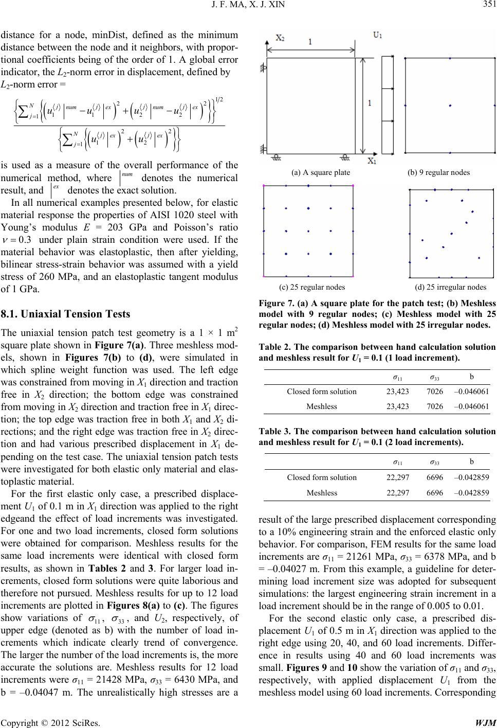 J. F. MA, X. J. XIN Copyright © 2012 SciRes. WJM 351 distance for a node, minDist, defined as the minimum distance between the node and it neighbors, with propor- tional coefficients being of the order of 1. A global error indicator, the L2-norm error in displacement, defined by L2-norm error = 1 22 1122 1 22 12 1 2 Nnum exnum ex j jjj Nex e j jx j j uuuu uu is used as a measure of the overall performance of the numerical method, where num denotes the numerical result, and ex denotes the exact solution. In all numerical examples presented below, for elastic material response the properties of AISI 1020 steel with Young’s modulus E = 203 GPa and Poisson’s ratio 0.3 under plain strain condition were used. If the material behavior was elastoplastic, then after yielding, bilinear stress-strain behavior was assumed with a yield stress of 260 MPa, and an elastoplastic tangent modulus of 1 GPa. 8.1. Uniaxial Tension Tests The uniaxial tension patch test geometry is a 1 × 1 m2 square plate shown in Figure 7(a). Three meshless mod- els, shown in Figures 7(b) to (d), were simulated in which spline weight function was used. The left edge was constrained from moving in X1 direction and traction free in X2 direction; the bottom edge was constrained from moving in X2 direction and traction free in X1 direc- tion; the top edge was traction free in both X1 and X2 di- rections; and the right edge was traction free in X2 direc- tion and had various prescribed displacement in X1 de- pending on the test case. The uniaxial tension patch tests were investigated for both elastic only material and elas- toplastic material. For the first elastic only case, a prescribed displace- ment U1 of 0.1 m in X1 direction was applied to the right edgeand the effect of load increments was investigated. For one and two load increments, closed form solutions were obtained for comparison. Meshless results for the same load increments were identical with closed form results, as shown in Tables 2 and 3. For larger load in- crements, closed form solutions were quite laborious and therefore not pursued. Meshless results for up to 12 load increments are plotted in Figures 8(a) to (c). The figures show variations of 11 , 33 , and U2, respectively, of upper edge (denoted as b) with the number of load in- crements which indicate clearly trend of convergence. The larger the number of the load increments is, the more accurate the solutions are. Meshless results for 12 load increments were σ11 = 21428 MPa, σ33 = 6430 MPa, and b = –0.04047 m. The unrealistically high stresses are a (a) A square plate (b) 9 regular nodes (c) 25 regular nodes (d) 25 irregular nodes Figure 7. (a) A square plate for the patch test; (b) Meshless model with 9 regular nodes; (c) Meshless model with 25 regular nodes; (d) Meshless model with 25 irregular nodes. Table 2. The comparison between hand calculation solution and meshless result for U1 = 0.1 (1 load increment). σ11 σ33 b Closed form solution 23,423 7026 –0.046061 Meshless 23,423 7026 –0.046061 Table 3. The comparison between hand calculation solution and meshless result for U1 = 0.1 (2 load increments). σ11 σ33 b Closed form solution 22,297 6696 –0.042859 Meshless 22,297 6696 –0.042859 result of the large prescribed displacement corresponding to a 10% engineering strain and the enforced elastic only behavior. For comparison, FEM results for the same load increments are σ11 = 21261 MPa, σ33 = 6378 MPa, and b = –0.04027 m. From this example, a guideline for deter- mining load increment size was adopted for subsequent simulations: the largest engineering strain increment in a load increment should be in the range of 0.005 to 0.01. For the second elastic only case, a prescribed dis- placement U1 of 0.5 m in X1 direction was applied to the right edge using 20, 40, and 60 load increments. Differ- ence in results using 40 and 60 load increments was small. Figures 9 and 10 show the variation of σ11 and σ33, respectively, with applied displacement U1 from the meshless model using 60 load increments. Corresponding  J. F. MA, X. J. XIN Copyright © 2012 SciRes. WJM 352 21000 21500 22000 22500 23000 23500 24000 0510 15 Number of load increments σ 11 (MPa) Meshless Closed form (a) 6400 6500 6600 6700 6800 6900 7000 7100 05101 Number of load increments σ 33 (MPa) Meshless Closed form (b) -0.047 -0.046 -0.045 -0.044 -0.043 -0.042 -0.041 -0.04 -0.039 0510 15 Number of load increments U 2 of upper edge (m) Meshless Closed form (c) Figure 8. (a) The convergence test of meshless method for Cauchy stress σ11 for elastic case; (b) The convergence test of meshless method for Cauchy stress σ33 for elastic case; (c) The convergence test of meshless method for displacement of upper edge for elastic case. FEM simulation was carried out for comparison. Good agreement between the meshless results and FEM results is evident. Nonlinear behavior, although not strong, is 0 10000 20000 30000 40000 50000 60000 70000 80000 90000 100000 00.1 0.2 0.3 0.40.5 0.6 U 1 (m) σ 11 (MPa) FEM Meshless Figure 9. FEM results versus meshless results of Cauchy stress σ11 for uniaxial tension simulation for elastic case. 0 5000 10000 15000 20000 25000 30000 00.1 0.2 0.3 0.4 0.5 0.6 U 1 (m) σ 33 (MPa) FEM Meshless Figure 10. FEM results versus meshless results of Cauchy stress σ11 for uniaxial tension simulation for elastic case. noticeable. For elastoplastic material behavior, since closed form results are not available, FEM results were used as the basis for comparison. For the first elastoplastic case, a prescribed displacement U1 of 0.1 m in X1 direction was applied to the right edge under different number of load increments. Figures 11(a) to (c) show variations of σ11, σ33, and U2, respectively, of the upper edge (denoted as b) with the number of load increments, together with the corresponding FEM results. The figures indicate trend of convergence, and con- verged values for FEM and meshless method are close to each other. The meshlessresults for 12 load increments are σ11 = 426 MPa, σ33 = 212 MPa, and b = –0.09009 m. The corresponding results of FEM with 12 load incre- ments are σ11 = 426 MPa, σ33 = 212 MPa, and b = –0.08978 m. It is noted that the current meshless method is based on Green-Naghdi’s theory, while FEM is based on E. H. Lee’s theory [2]. The differences between mesh- less results and FEM results show that large deformation  J. F. MA, X. J. XIN Copyright © 2012 SciRes. WJM 353 300 320 340 360 380 400 420 440 460 480 500 0510 15 number of load increments σ 11 (MPa) Meshless FEM (a) 100 120 140 160 180 200 220 240 260 280 300 0510 15 number of load increments σ 33 (MPa) Meshless FEM (b) -0.16 -0.14 -0.12 -0.1 -0.08 -0.06 -0.04 -0.02 0 051015 number of load increments U 2 of upper edge (m) Meshless FEM (c) Figure 11. (a) The convergence test of FEM results and meshless results for Cauchy stress σ11 for elastoplastic case; (b) The convergence test of FEM results and meshless results for Cauchy stress σ33 for elastoplastic case; (c) The convergence test of FEM results and meshless results for displacement of upper edge for elastoplastic case. elastoplasticity theories may have some influence on the numerical results. For the second elastoplastic case, a prescribed dis- placement U1 of 0.5 m in X1 direction was applied to the right edge using 60 load increments. Figures 12 and 13 show the variation of σ11 and σ33, respectively, with ap- plied displacement U1 from the meshless model and FEM model. Good agreement between the meshless re- sults and FEM results is evident. 8.2. The Shear Tests The shear patch test geometry is a 1 × 1 m2 square plate shown in Figure 14. Three meshless models, shown in Figures 14(b) to (d), with spline weight function were simulated. The motion of the square was described by 112 XX and 22 X . Three values of , 0.1, 0.5 and 1.0, were simulated. For all three models, pre- scribed displacements were applied to all edges of the plate. For the shear tests, both elastic only material and elastoplastic material were investigated. 0 100 200 300 400 500 600 700 800 900 00.1 0.2 0.3 0.4 0.50.6 U 1 (m) σ 11 (MPa) FEM Meshless Figure 12. FEM results versus meshless results of σ11 for uniaxial tension simulation for elastoplastic case. 0 50 100 150 200 250 300 350 400 450 00.1 0.20.30.40.5 0.6 U 1 (m) σ 33 (MPa) FEM Meshless Figure 13. FEM versus meshless results of Cauchy stress σ33 for uniaxial tension simulation for elastoplastic case.  J. F. MA, X. J. XIN Copyright © 2012 SciRes. WJM 354 (a) A square plate (b) 9 regular nodes (c) 25 regular nodes (d) 25 irregular nodes Figure 14. (a) A square plate for the shear tests; (b) Meshless model with 9 regular nodes; (c) Meshless model with 25 regular nodes; (d) Meshless model with 25 irregular nodes. For elastic only material behavior, analytical results in terms of the Cauchy stress using Jaumann rate for this problem are given as [56]: 1122 1cos (72) 12 sin (73) The constitutive equation in terms of the Jaumann rate is given by: Ttrace 2 JJJ WW σσ σσ ID (74) where D is the rate-of-deformation tensor and 0.1 W is the spin tensor, and the superscript, J, denotes that the material constants are used with the Jaumann rate. For the first elastic only shear test with 0.1 , the L2-norms between meshless results and analytical solu- tions for the 9 node, 25 node regular, and 25 node ir- regular models are 3.2 × 10⁻¹⁶, 2.6 × 10⁻¹⁸, and 3.6 × 10⁻¹⁷ respectively. The stresses for all three models are σ11 = 390 MPa, σ22 = –391.48 MPa, σ12 = 7794.88 MPa which are practically identical with the analytical solu- tion using Jaumann rate: σ11 = 390 MPa, σ22 = –390 MPa, σ12 = 7794.68 MPa. Note that although it is pure shear loading, non-zero normal stresses in the X1 and X2 direc- tions are present due to large deformation. For the second elastic only shear test with 0.5 , the L2-norms between meshless results and analytical solutions for the 9 node, 25 node regular, and 25 node irregular models are 6.2 × 10⁻¹⁶, 5.5 × 10⁻¹⁸, and 4.7 × 10⁻¹⁶ respectively. The stresses for all three models are σ11 = 9560 MPa, σ22 = –9555 MPa, σ12 = 37431 MPa which are practically identical with the analytical solu- tion using Jaumann rate: σ11 = 9557 MPa, σ22 =–9557 MPa, σ12 = 37432 MPa. For the third elastic only shear test, Figures 15(a)-(c) show the variation of normal stresses σ11, σ22, and shear stress σ12 with increasing up to 3.0 from meshless model, together with the analytical results. These three figures reveal that the meshless results match the ana- lytical results almost identically. (a) (b) (c) Figure 15. (a) Analytical versus meshless results of Cauchy stress σ11 of the shear test for elastic case; (b) Analytical versus meshless results of Cauchy stress σ22 of the shear test for elastic case; (c) Analytical versus meshless results of Cauchy stress σ12 of the shear test for elastic case. 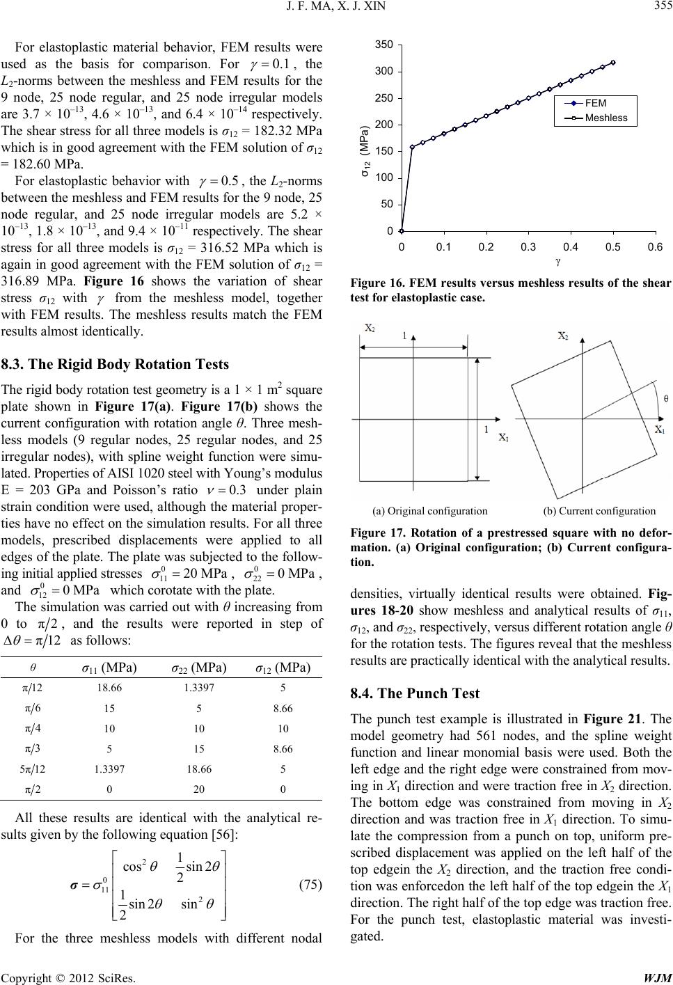 J. F. MA, X. J. XIN Copyright © 2012 SciRes. WJM 355 For elastoplastic material behavior, FEM results were used as the basis for comparison. For 0.1 , the L2-norms between the meshless and FEM results for the 9 node, 25 node regular, and 25 node irregular models are 3.7 × 10⁻¹³, 4.6 × 10⁻¹³, and 6.4 × 10⁻¹⁴ respectively. The shear stress for all three models is σ12 = 182.32 MPa which is in good agreement with the FEM solution of σ12 = 182.60 MPa. For elastoplastic behavior with 0.5 , the L2-norms between the meshless and FEM results for the 9 node, 25 node regular, and 25 node irregular models are 5.2 × 10⁻¹³, 1.8 × 10⁻¹³, and 9.4 × 10⁻¹¹ respectively. The shear stress for all three models is σ12 = 316.52 MPa which is again in good agreement with the FEM solution of σ12 = 316.89 MPa. Figure 16 shows the variation of shear stress σ12 with from the meshless model, together with FEM results. The meshless results match the FEM results almost identically. 8.3. The Rigid Body Rotation Tests The rigid body rotation test geometry is a 1 × 1 m2 square plate shown in Figure 17(a). Figure 17(b) shows the current configuration with rotation angle θ. Three mesh- less models (9 regular nodes, 25 regular nodes, and 25 irregular nodes), with spline weight function were simu- lated. Properties of AISI 1020 steel with Young’s modulus E = 203 GPa and Poisson’s ratio 0.3 under plain strain condition were used, although the material proper- ties have no effect on the simulation results. For all three models, prescribed displacements were applied to all edges of the plate. The plate was subjected to the follow- ing initial applied stresses 0 11 20MPa , 0 22 0MPa , and 0 12 0MPa which corotate with the plate. The simulation was carried out with θ increasing from 0 to π2, and the results were reported in step of π12 as follows: θ σ11 (MPa) σ22 (MPa) σ12 (MPa) π12 18.66 1.3397 5 π6 15 5 8.66 π4 10 10 10 π3 5 15 8.66 5π12 1.3397 18.66 5 π2 0 20 0 All these results are identical with the analytical re- sults given by the following equation [56]: 2 0 11 2 1 cossin 2 2 1sin 2sin 2 σ (75) For the three meshless models with different nodal 0 50 100 150 200 250 300 350 00.1 0.2 0.3 0.4 0.5 0.6 γ σ 12 (MPa) FEM Meshless Figure 16. FEM results versus meshless results of the shear test for elastoplastic case. (a) Original configuration (b) Current configuration Figure 17. Rotation of a prestressed square with no defor- mation. (a) Original configuration; (b) Current configura- tion. densities, virtually identical results were obtained. Fig- ures 18-20 show meshless and analytical results of σ11, σ12, and σ22, respectively, versus different rotation angle θ for the rotation tests. The figures reveal that the meshless results are practically identical with the analytical results. 8.4. The Punch Test The punch test example is illustrated in Figure 21. The model geometry had 561 nodes, and the spline weight function and linear monomial basis were used. Both the left edge and the right edge were constrained from mov- ing in X1 direction and were traction free in X2 direction. The bottom edge was constrained from moving in X2 direction and was traction free in X1 direction. To simu- late the compression from a punch on top, uniform pre- scribed displacement was applied on the left half of the top edgein the X2 direction, and the traction free condi- tion was enforcedon the left half of the top edgein the X1 direction. The right half of the top edge was traction free. For the punch test, elastoplastic material was investi- gated. 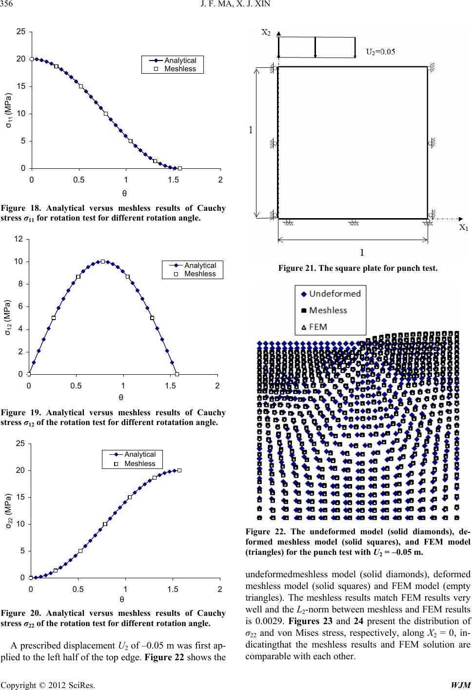 J. F. MA, X. J. XIN Copyright © 2012 SciRes. WJM 356 0 5 10 15 20 25 00.511.52 θ σ 11 (MPa) Analytical Meshless Figure 18. Analytical versus meshless results of Cauchy stress σ11 for rotation test for different rotation angle. 0 2 4 6 8 10 12 00.511.52 θ σ 12 (MPa) Analytical Meshless Figure 19. Analytical versus meshless results of Cauchy stress σ12 of the rotation test for different rotatation angle. 0 5 10 15 20 25 00.511.52 σ 22 (MPa) Analytical Meshless Figure 20. Analytical versus meshless results of Cauchy stress σ22 of the rotation test for different rotation angle. A prescribed displacement U2 of –0.05 m was first ap- plied to the left half of the top edge. Figure 22 shows the Figure 21. The square plate for punch test. Figure 22. The undeformed model (solid diamonds), de- formed meshless model (solid squares), and FEM model (triangles) for the punch test with U2 = –0.05 m. undeformedmeshless model (solid diamonds), deformed meshless model (solid squares) and FEM model (empty triangles). The meshless results match FEM results very well and the L2-norm between meshless and FEM results is 0.0029. Figures 23 and 24 present the distribution of σ22 and von Mises stress, respectively, along X2 = 0, in- dicatingthat the meshless results and FEM solution are comparable with each other. 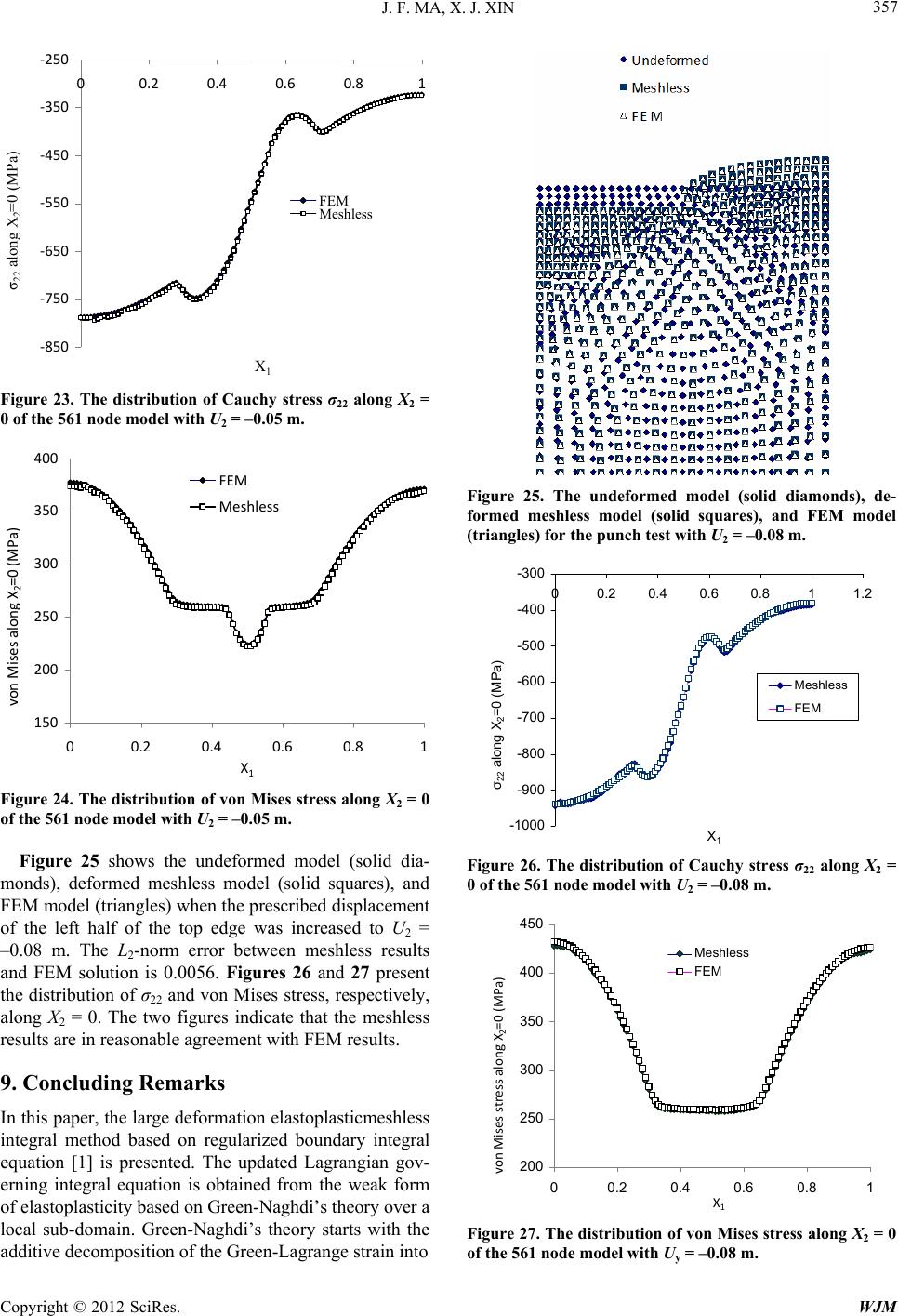 J. F. MA, X. J. XIN Copyright © 2012 SciRes. WJM 357 ‐850 ‐750 ‐650 ‐550 ‐450 ‐350 ‐250 00.2 0.4 0.6 0.81 X 1 σ 22 along X 2 =0 (MPa) FEM Meshless Figure 23. The distribution of Cauchy stress σ22 along X2 = 0 of the 561 node model with U2 = –0.05 m. 150 200 250 300 350 400 00.2 0.4 0.6 0.81 X 1 vonMisesalongX 2 =0(MPa) FEM Meshless Figure 24. The distribution of von Mises stress along X2 = 0 of the 561 node model with U2 = –0.05 m. Figure 25 shows the undeformed model (solid dia- monds), deformed meshless model (solid squares), and FEM model (triangles) when the prescribed displacement of the left half of the top edge was increased to U2 = –0.08 m. The L2-norm error between meshless results and FEM solution is 0.0056. Figures 26 and 27 present the distribution of σ22 and von Mises stress, respectively, along X2 = 0. The two figures indicate that the meshless results are in reasonable agreement with FEM results. 9. Concluding Remarks In this paper, the large deformation elastoplasticmeshless integral method based on regularized boundary integral equation [1] is presented. The updated Lagrangian gov- erning integral equation is obtained from the weak form of elastoplasticity based on Green-Naghdi’s theory over a local sub-domain. Green-Naghdi’s theory starts with the additive decomposition of the Green-Lagrange strain into Figure 25. The undeformed model (solid diamonds), de- formed meshless model (solid squares), and FEM model (triangles) for the punch test with U2 = –0.08 m. -1000 -900 -800 -700 -600 -500 -400 -300 00.2 0.4 0.6 0.811.2 X 1 σ 22 along X 2 =0 (MPa) Meshless FEM Figure 26. The distribution of Cauchy stress σ22 along X2 = 0 of the 561 node model with U2 = –0.08 m. 200 250 300 350 400 450 00.2 0.4 0.6 0.81 X 1 vonMisesstressalongX 2 =0(MPa) Meshless FEM Figure 27. The distribution of von Mises stress along X2 = 0 of the 561 node model with Uy = –0.08 m. 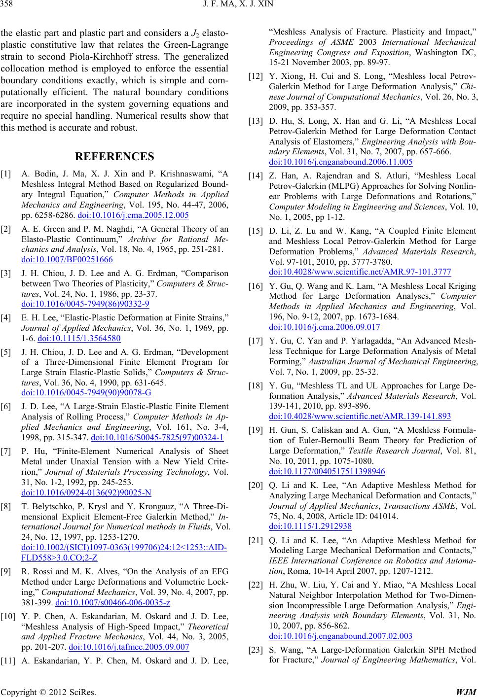 J. F. MA, X. J. XIN Copyright © 2012 SciRes. WJM 358 the elastic part and plastic part and considers a J2 elasto- plastic constitutive law that relates the Green-Lagrange strain to second Piola-Kirchhoff stress. The generalized collocation method is employed to enforce the essential boundary conditions exactly, which is simple and com- putationally efficient. The natural boundary conditions are incorporated in the system governing equations and require no special handling. Numerical results show that this method is accurate and robust. REFERENCES [1] A. Bodin, J. Ma, X. J. Xin and P. Krishnaswami, “A Meshless Integral Method Based on Regularized Bound- ary Integral Equation,” Computer Methods in Applied Mechanics and Engineering, Vol. 195, No. 44-47, 2006, pp. 6258-6286. 0doi:10.1016/j.cma.2005.12.005 [2] A. E. Green and P. M. Naghdi, “A General Theory of an Elasto-Plastic Continuum,” Archive for Rational Me- chanics and Analysis, Vol. 18, No. 4, 1965, pp. 251-281. 1doi:10.1007/BF00251666 [3] J. H. Chiou, J. D. Lee and A. G. Erdman, “Comparison between Two Theories of Plasticity,” Computers & Struc- tures, Vol. 24, No. 1, 1986, pp. 23-37. 2doi:10.1016/0045-7949(86)90332-9 [4] E. H. Lee, “Elastic-Plastic Deformation at Finite Strains,” Journal of Applied Mechanics, Vol. 36, No. 1, 1969, pp. 1-6. 3doi:10.1115/1.3564580 [5] J. H. Chiou, J. D. Lee and A. G. Erdman, “Development of a Three-Dimensional Finite Element Program for Large Strain Elastic-Plastic Solids,” Computers & Struc- tures, Vol. 36, No. 4, 1990, pp. 631-645. 4doi:10.1016/0045-7949(90)90078-G [6] J. D. Lee, “A Large-Strain Elastic-Plastic Finite Element Analysis of Rolling Process,” Computer Methods in Ap- plied Mechanics and Engineering, Vol. 161, No. 3-4, 1998, pp. 315-347. 5doi:10.1016/S0045-7825(97)00324-1 [7] P. Hu, “Finite-Element Numerical Analysis of Sheet Metal under Unaxial Tension with a New Yield Crite- rion,” Journal of Materials Processing Technology, Vol. 31, No. 1-2, 1992, pp. 245-253. 6doi:10.1016/0924-0136(92)90025-N [8] T. Belytschko, P. Krysl and Y. Krongauz, “A Three-Di- mensional Explicit Element-Free Galerkin Method,” In- ternational Journal for Numerical methods in Fluids, Vol. 24, No. 12, 1997, pp. 1253-1270. 7doi:10.1002/(SICI)1097-0363(199706)24:12<1253::AID- FLD558>3.0.CO;2-Z [9] R. Rossi and M. K. Alves, “On the Analysis of an EFG Method under Large Deformations and Volumetric Lock- ing,” Computational Mechanics, Vol. 39, No. 4, 2007, pp. 381-399. 8doi:10.1007/s00466-006-0035-z [10] Y. P. Chen, A. Eskandarian, M. Oskard and J. D. Lee, “Meshless Analysis of High-Speed Impact,” Theoretical and Applied Fracture Mechanics, Vol. 44, No. 3, 2005, pp. 201-207. 9doi:10.1016/j.tafmec.2005.09.007 [11] A. Eskandarian, Y. P. Chen, M. Oskard and J. D. Lee, “Meshless Analysis of Fracture. Plasticity and Impact,” Proceedings of ASME 2003 International Mechanical Engineering Congress and Exposition, Washington DC, 15-21 November 2003, pp. 89-97. [12] Y. Xiong, H. Cui and S. Long, “Meshless local Petrov- Galerkin Method for Large Deformation Analysis,” Chi- nese Journal of Computational Mechanics, Vol. 26, No. 3, 2009, pp. 353-357. [13] D. Hu, S. Long, X. Han and G. Li, “A Meshless Local Petrov-Galerkin Method for Large Deformation Contact Analysis of Elastomers,” Engineering Analysis with Bou- ndary Elements, Vol. 31, No. 7, 2007, pp. 657-666. 1doi:10.1016/j.enganabound.2006.11.005 [14] Z. Han, A. Rajendran and S. Atluri, “Meshless Local Petrov-Galerkin (MLPG) Approaches for Solving Nonlin- ear Problems with Large Deformations and Rotations,” Computer Modeling in Engineering and Sciences, Vol. 10, No. 1, 2005, pp 1-12. [15] D. Li, Z. Lu and W. Kang, “A Coupled Finite Element and Meshless Local Petrov-Galerkin Method for Large Deformation Problems,” Advanced Materials Research, Vol. 97-101, 2010, pp. 3777-3780. 1doi:10.4028/www.scientific.net/AMR.97-101.3777 [16] Y. Gu, Q. Wang and K. Lam, “A Meshless Local Kriging Method for Large Deformation Analyses,” Computer Methods in Applied Mechanics and Engineering, Vol. 196, No. 9-12, 2007, pp. 1673-1684. 1doi:10.1016/j.cma.2006.09.017 [17] Y. Gu, C. Yan and P. Yarlagadda, “An Advanced Mesh- less Technique for Large Deformation Analysis of Metal Forming,” Australian Journal of Mechanical Engineering, Vol. 7, No. 1, 2009, pp. 25-32. [18] Y. Gu, “Meshless TL and UL Approaches for Large De- formation Analysis,” Advanced Materials Research, Vol. 139-141, 2010, pp. 893-896. 1doi:10.4028/www.scientific.net/AMR.139-141.893 [19] H. Gun, S. Caliskan and A. Gun, “A Meshless Formula- tion of Euler-Bernoulli Beam Theory for Prediction of Large Deformation,” Textile Research Journal, Vol. 81, No. 10, 2011, pp. 1075-1080. 1doi:10.1177/0040517511398946 [20] Q. Li and K. Lee, “An Adaptive Meshless Method for Analyzing Large Mechanical Deformation and Contacts,” Journal of Applied Mechanics, Transactions ASME, Vol. 75, No. 4, 2008, Article ID: 041014. 1doi:10.1115/1.2912938 [21] Q. Li and K. Lee, “An Adaptive Meshless Method for Modeling Large Mechanical Deformation and Contacts,” IEEE International Conference on Robotics and Automa- tion, Roma, 10-14 April 2007, pp. 1207-1212. [22] H. Zhu, W. Liu, Y. Cai and Y. Miao, “A Meshless Local Natural Neighbor Interpolation Method for Two-Dimen- sion Incompressible Large Deformation Analysis,” Engi- neering Analysis with Boundary Elements, Vol. 31, No. 10, 2007, pp. 856-862. 1doi:10.1016/j.enganabound.2007.02.003 [23] S. Wang, “A Large-Deformation Galerkin SPH Method for Fracture,” Journal of Engineering Mathematics, Vol.  J. F. MA, X. J. XIN Copyright © 2012 SciRes. WJM 359 71, No. 3, 2011, pp. 305-318. 1doi:10.1007/s10665-011-9455-7 [24] J. Chen, C. Pan, C. Wu and W. Liu, “Reproducing Kernel Particle Methods for Large Deformation Analysis of Non- Linear Structures,” Computer Methods in Applied Me- chanics and Engineering, Vol. 139, No. 1-4, 1996, pp. 195-227. 1doi:10.1016/S0045-7825(96)01083-3 [25] S. Jun, W. Liu and T. Belytschko, “Explicit Reproducing Kernel Particle Methods for Large Deformation Prob- lems,” International Journal for Numerical Methods in Engineering, Vol. 41, No. 1, 1998, pp. 137-166. 1doi:10.1002/(SICI)1097-0207(19980115)41:1<137::AID- NME280>3.0.CO;2-A [26] K. Liew, T. Ng and Y. Wu, “Meshfree Method for Large Deformation Analysis—A Reproducing Kernel Particle Approach,” Engineering Structures, Vol. 24, No. 5, 2002, pp. 543-551. 2doi:10.1016/S0141-0296(01)00120-1 [27] D. Li, J. Xu and W. Kang, “Applying Element-Free Gal- erkin Method to Simulate Die Forging Problems,” Advan- ced Materials Research, Vol. 139-141, 2010, pp. 1174-1177. 2doi:10.4028/www.scientific.net/AMR.139-141.1174 [28] W. Quak, A. van den Boogaard and J. Huétink, “Mesh- less Methods and Forming Processes,” International Journal of Material Forming, Vol. 2, No. S1, 2009, pp. 585-588. [29] J. Ma, X. J. Xin and P. Krishnaswami, “An Elastoplastic Meshless Integral Method Based on Regularized Boun- dary Integral Equation,” Computer Methods in Applied Mechanics and Engineering, Vol. 197, No. 51-52, 2008, pp. 4774-4788. 2doi:10.1016/j.cma.2008.06.019 [30] J. Ma, “Application of Meshless Integral Method to Metal Forming,” Proceedings of the ASME Design Engineering Technical Conference, Montreal, 15-18 August 2010, pp. 141-151. [31] S. N. Atluri, J. Sladeck, V. Sladeck and T. Zhu, “The Local Boundary Integral Equation (LBIE) and Its Mesh- less Implementation for Linear Elasticity,” Computa- tional Mechanics, Vol. 25, No. 2-3, 2000, pp. 180-198. 2doi:10.1007/s004660050468 [32] A. H. Stroud and D. Secrest, “Gaussian Quadrature For- mulas,” Prentice-Hall, Upper Saddle River, 1966. [33] Y. Y. Lu, T. Belytschko and L. Gu, “A New Implementa- tion of the Element Free Galerkin Method,” Computer Methods in Applied Mechanics and Engineering, Vol. 113, No. 3-4, 1994, pp. 397-414. 2doi:10.1016/0045-7825(94)90056-6 [34] T. Belytschko, Y. Y. Lu and L. Gu, “Element Free Gal- erkin Method,” International Journal for Numerical Me- thods in Engineering, Vol. 37, No. 2, 1994, pp. 229-256. 2doi:10.1002/nme.1620370205 [35] L. Gavete, J. J. Benito, S. Falcon and A. Ruiz, “Imple- mentation of Essential Boundary Conditions in a Mesh- less Method,” Communications in Numerical Methods. Engineering, Vol. 16, No. 6, 2000, pp. 409-421. 2doi:10.1002/1099-0887(200006)16:6<409::AID-CNM34 9>3.0.CO;2-Z [36] T. Zhu and S. N. Atluri, “A Modified Collocation Method and a Penalty Foumulation for Enforcing the Essential Boundary Conditions in the Element Free Galerkin Me- thod,” Computational Mechanics, Vol. 21, No. 3, 1998, pp. 211-222. 2doi:10.1007/s004660050296 [37] D. N. Arnold, F. Brezzi, B. Cockburn and L. D. Marini, “Unified Analysis of Discontinuous Galerkin Methods for Elliptic Problems,” SIMA Journal on Numerical Analysis, Vol. 39, No. 5, 2002, pp. 1749-1779. 2doi:10.1137/S0036142901384162 [38] D. Hegen, “Element-Free Galerkin Methods in Combina- tion with Finite Element Approaches,” Computer Meth- ods in Applied Mechanics and Engineering, Vol. 19, No. 1, 1996, pp. 120-135. [39] J. Gosz and W. K. Liu, “Admissible Approximations for Essential Boundary Conditions in the Reproducing Ker- nel Particle Method,” Computational Mechanics, Vol. 19, No. 2, 1996, pp. 120-135. 2doi:10.1007/BF02824850 [40] F. C. Gunther and W. K. Liu, “Implementation of Bound- ary Conditions for Meshless Methods,” Computer Meth- ods in Applied Mechanics and Engineering, Vol. 163, No. 1-4, 1998, pp. 205-230. 3doi:10.1016/S0045-7825(98)00014-0 [41] C. A. M. Duarte and J. T. Oden, “An h-p Adaptive Me- thod Using Clouds,” Computer Methods in Applied Me- chanics and Engineering, Vol. 139, No. 1-4, 1996, pp. 237-262. 3doi:10.1016/S0045-7825(96)01085-7 [42] Y. Y. Lu, T. Belytschko and M. Tabbara, “Element-Free Galerkin Method for Wave Propagation and Dynamic Fracture,” Computer Methods in Applied Mechanics and Engineering, Vol. 126, No. 1-2, 1995, pp. 131-153. 3doi:10.1016/0045-7825(95)00804-A [43] X. Zhang, X. Liu, M. W. Lu and Y. Chen, “Imposition of Essential Boundary Conditions by Displacement Con- straint Equations in Meshless Methods,” Communications in Numerical Methods in Engineering, Vol. 17, No. 3, 2001, pp. 165-178. 3doi:10.1002/cnm.395 [44] T. Zhu and S. N. Atluri, “A Modified Collocation Method and a Penalty Foumulation for Enforcing the Essential Boundary Conditions in the Element Free Galerkin Me- thod,” Computational Mechanics, Vol. 21, No. 3, 1998, pp. 211-222. 3doi:10.1007/s004660050296 [45] G. J. Wagner and W. K. Liu, “Application of Essential Boundary Conditions in Mesh-Free Methods: A Corre- cted Collocation Method,” International Journal for Nu- merical Methods in Engineering, Vol. 47, No. 8, 2000, pp. 1367-1379. 3doi:10.1002/(SICI)1097-0207(20000320)47:8<1367::AID -NME822>3.0.CO;2-Y [46] C. C. Wu and M. E. Plesha, “Essential Boundary Condi- tion Enforcement in Meshless Methods: Boundary Flux Collocation Method,” International Journal for Numeri- cal Methods in Engineering, Vol. 53, No. 3, 2002, pp. 499-514. 3doi:10.1002/nme.267 [47] T. Belytschko, Y. Y. Lu and L. Gu, “Element Free Gal- erkin Method,” International Journal for Numerical Me- thods in Engineering, Vol. 37, No. 2, 1994, pp. 229-256. 3doi:10.1002/nme.1620370205 [48] P. Krysl and T. Belytschko, “Analysis of Thin Plates by the Element-Free Galerkin Method,” Computational Me-  J. F. MA, X. J. XIN Copyright © 2012 SciRes. WJM 360 chanics, Vol. 17, No. 1, 1998, pp. 26-35. [49] W. K. Liu and Y. Chen, “Wavelet and Multiple Scale Reproducing Kernel Methods,” International Journal for Numerical Methods in Fluids, Vol. 21, No. 10, 1995, pp. 901-931. [50] N. R. Aluru, “A Reproducing Kernel Particle Method for Meshless Analysis of Microelectromechanical Systems,” Computational Mechanics, Vol. 23, No. 4, 1999, pp. 324- 338. 3doi:10.1007/s004660050413 [51] J. S. Chen, C. Pan and C. T. Wu, “A Lagrangian Repro- ducing Kernel Particle Method for Metal Forming Analy- sis,” Computational Mechanics, Vol. 22, No. 3, 1998, pp. 289-338. 3doi:10.1007/s004660050361 [52] J. S. Chen, C. Pan, C. T. Wu and W. K. Liu, “Reproduc- ing Kernel Particle Methods for Large Deformation Ana- lysis of Non-Linear Structures,” Computer Methods in Applied Mechanics and Engineering, Vol. 139, No. 1-4, 1996, pp. 195-227. doi:10.1016/S0045-7825(96)01083-3 [53] T. Zhu, J.-D. Zhang and S. N. Atluri, “A Local Boundary Integral Equation (LBIE) Method in Computational Me- chanics, and a Meshless Discretization Approach,” Com- putational Mechanics, Vol. 21, No. 3, 1998, pp. 223-235. 4doi:10.1007/s004660050297 [54] J. Sladek, V. Sladeck and R. Van Keer, “Meshless Local Boundary Integral Equation for 2D Elastodynamic Prob- lems,” International Journal for Numerical Methods in Engineering, Vol. 57, No. 2, 2003, pp. 235-249. 4doi:10.1002/nme.675 [55] S. Long and Q. Zhang, “Analysis of Thin Plates by the Local Boundary Integral Equation (LBIE) Method,” En- gineering Analysis with Boundary Elements, Vol. 26, No. 8, 2002, pp. 707-718. 4doi:10.1016/S0955-7997(02)00025-5 [56] T. Belytschko, W. K. Liu and B. Moran, “Nonlinear Fi- nite Elements for Continua and Structures,” John Wiley & Sons, Ltd., Chichester, 2000.
|