Applied Mathematics
Vol.05 No.13(2014), Article ID:47989,9 pages
10.4236/am.2014.513203
Influence of the Domain Boundary on the Speeds of Traveling Waves
Lanxiang Ma1, Jiale Tan2
1Ningbo Shentong Energy Co., Ltd., Ningbo, China
2Department of Mathematics, Tongji University, Shanghai, China
Email: lanxiangma@163.com, jialetan5293@gmail.com
Copyright © 2014 by authors and Scientific Research Publishing Inc.
This work is licensed under the Creative Commons Attribution International License (CC BY).
http://creativecommons.org/licenses/by/4.0/


Received 30 April 2014; revised 5 June 2014; accepted 15 June 2014
ABSTRACT
Let H > 0 be a constant, g ≥ 0 be a periodic function and . We consider a curvature flow equation V = κ + A in Ω, where for a simple curve
 , V denotes its normal velocity, κ denotes its curvature and A > 0 is a constant. [1] proved that this equation has a periodic traveling wave U, and that the average speed c of U is increasing in A and H, decreasing in max g' when the scale of g is sufficiently small. In this paper we study the dependence of c on A, H, max g' and on the period of g when the scale of g is large. We show that similar results as [1] hold in certain weak sense.
Keywords:
Curvature Flow Equation, Traveling Wave, Average Speed, Spatial Heterogeneity

1. Introduction
We study traveling waves for a curvature-driven motion of plane curves in a band domain Ω. The law of motion of the curve is given by
 (1)
(1)
where  is a simple, smooth curve, V denotes its normal velocity,
  denotes its curvature and A is a positive constant representing a driving force. The band domain Ω is defined as the following. Set
 (2)
(2)
For some  we define

where  is a constant and
  for some
  (see Figure 1). Denote the left (resp. right) boundary of Ω by
  (resp.
 ).
).
By a solution of (1) we mean a time-dependent simple, smooth curve  in Ω which satisfies (1) and contacts
  perpendicularly. Equation (1) appears as a certain singular limit of an Allen-Cahn type nonlinear diffusion equation under the Neumann boundary conditions. The curve
  represents the interface between two different phases (see, e.g., [1] -[4] for details). In physics, chemistry and many other fields, an interface may propagate in a domain with obstacles, say, with obstacles lying in several lines. The motion of the interface between two adjacent lines is then like the propagation of
  in Ω in our problem. Hence the undulation of the boundary of Ω can be regarded as effect of obstacles and so it can be in any size. [1] studied the homogenization limit of this problem (as
 ), we will consider the case where p is large.
To avoid sign confusion, the normal to the curve  will always be chosen toward the upper region, and the sign of the normal velocity V and the curvature
  will be understood in accordance with this choice of the normal direction. Consequently,
  is negative at those points where the curve is concave while it is positive where the curve is convex (see Figure 1).
In the case where  is expressed as a graph of a function
  at each time t. Let
  be the x-coordinates of the end points of
  lying on
 ,
,  , respectively. In other words,
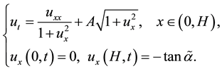
  . Now (1) is equivalent to
 (3)
(3)
with the boundary conditions
 (4)
(4)
with . The condition
  in the definition
  prevent
 from developing singularities near the boundary
  (cf. [1] ). Denote
 (5)
(5)
and call  the maximum opening angle of
 , or, of g. Then
  for
for .
.
Definition 1 A solution  for some
  (also write as
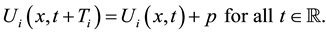
  for simplicity) of (3)-(4) is called a periodic traveling wave if it satisfies
 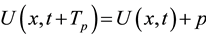 for some
 . Its average speed is defined by
 (6)
(6)
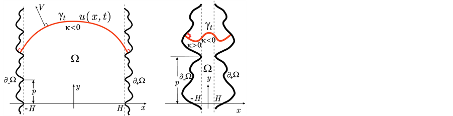
Figure 1. Domain Ω (the left one has fine boundaries, the right one has coarse boundaries).
In [1] the authors proved that, under the condition , the problem (3)-(4) has a periodic traveling wave
 , it is unique under the normalization condition
  and
and
 (7)
(7)
for all  and x where U is defined. In addition, [1] studied the homogenization limit of the average speed c.
Theorem A (Theorem 2.3 in [1] ). Assume that . Let
. Let  be the periodic traveling wave of (3)-(4) with average speed
 . Then
 (8)
(8)
where  is the constant determined uniquely by
 (9)
(9)
and M is a positive constant independent of p. Moreover  satisfies
 (10)
(10)
Theorem A gives the dependence of c on A, H and  near the homogenization limit (as
 ). It is known that in the study of spatially heterogeneous problems, homogenization is a powerful method when the spatial heterogeneity is fine (for example,
  in our problem) (cf. [5] [6] ). On the contrary, the mathematical analysis is completely different and very difficult when the spatial heterogeneity is coarse (for example,
  is large in our problem). How does the traveling wave U and its average speed c in our problem depend on the parameters
  and p when p is large? This is an interesting problem in physics and is also a challenging one in mathematics. Some mathematicians from Japan and France have been working on it for several years, but yet very little is known so far. Our main purpose in this paper is to study this problem by analytic and numerical methods, and try to give some answers.
This paper is arranged as the following. In section 2 we list some notations and present our main theorem. In section 3 we prove the main theorem. In subsection 3.1 we prove that  is increasing in A; in subsection 3.2 we prove that
  is increasing in some increasing sequence
 ; in subsection 3.3 we prove that
  is increasing in some decreasing sequence
 . Finally, in section 4 we present some numerical simulation results, including the dependence of c on the period p of
 .
.
2. Notations and Main Results
We list some notations for convenience. For any ,
,  ,
,  and
and , denote


 (11)
(11)

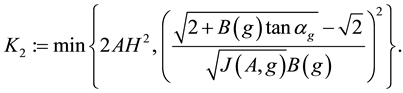
Clearly, N depends on  and K1, K2 depend on
 . Finally, for any
 ,
,  ,
,  , denote

Here is an example, let ,
,  ,
,  , then we have

It is easily seen that
 (12)
(12)
 (13)
(13)
Therefore, if  or
or  holds, then
 .
.
The following is our main result.
Main Theorem. Assume  and
and . Then
1)  is strictly increasing in A;
2) if , then
  is strictly increasing in k, where
  for
for ;
;
3) if , then
  is strictly increasing in
 , where N is given by (11),
  and
and
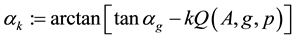 (14)
(14)
for .
.
We remark that 3) of the theorem mainly states the dependence of c on  but not on g itself. In fact, for
  defined by (14), the conclusion of 3) holds for any
  provided
  (with restrictions
 ,
, ), the exact shape of
  does not matter.
By the main theorem,  is increasing in continuously varying A, but it is increasing in H and decreasing in
  only in weak sense, that is, the monotonicity holds only for certain sequences. It turns out that the monotonicity for continuously varying H and
  is very difficult. In fact, we believe that
  is not true when p is large. This is quite different from the case where
 .
.
3. Proof of the Main Theorem
In this section, for any two solutions  and
and  of (3)-(4), when we write
  or
or  we mean that the inequality holds on the common domain where
  and
and  are defined.
3.1. Proof of Main Theorem 1
Assume that . For
. For , denote
  the (unique) periodic
traveling wave of (3)-(4) for , denote the x-span for each t by
 . Denote the time-period of
  by
by , that is,
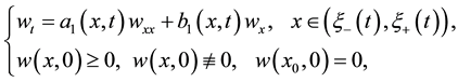
Let  be two times such that

for some . This is possible since
 . Define
for , where
Then  satisfies
where


are both bounded functions. We show that
 (15)
(15)
First by the maximum principle (see, for example, Theorem 2 in Chapter 3 in [7] ) we have
 (16)
(16)
This implies that the graph of  can not touch the graph of
  from below except on their end points. On the other hand, if the latter happens on the right boundary, that is, there exists
  such that
 , where
Then
 (17)
(17)
and so
 (18)
(18)
since, otherwise we have  for x near
  by Taylor’s formula. But this contradicts (16).
Using (17), (18), the fact  and using the equations of
  and
and  we have
Since the normal velocity V in (1) is expressed by

we see that at the point , the normal velocity V1 of U1 and the normal velocity V2 of U2 satisfies

This means that, in a small time-interval around , the graph of U1 moves along the boundary
  faster than the graph of U2. This, however, contradicts the fact
  and the assumption that
  . This proves (15).
Now taking  and
and  in (15) and using the definitions of
  we have

By the fact  in (7) we have
 . This implies that
  by the definition of c in (6). This proves 1) of the Main Theorem.
3.2. Dependence of c on H
In this subsection we study the dependence of c on H and prove Main Theorem 2). Since only H is varying, for simplicity, in this part we only indicate H but omit all the other parameters in the notations Ω, U, c, B, J, Ki, ∙∙∙.
Lemma 1 Assume that . Then for any
 , there holds
 (19)
(19)
Proof Let  such that
 . Denote
and
Then there exists  such that, for
 ,
,

Since  we have

and so
 (20)
(20)
For any , set
, set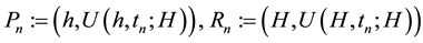 . Denote the straight line passing
  and
and  by
by  and denote its slope by
 , then by (20) we have
where 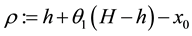 and
and . For any
 , since
 , the graph of
  must contact
  at some point in
 . If we denote the x-coordinate of the contact point by
 , then
 . Using (20) again we have
where . This proves (19). ,
Lemma 2 Assume that  and
and . Then
 , where
 .
.
Proof Since  we have by (12)
  and
and . The definition of
  and
and  imply that
  and so
So by Lemma 1 we have

Since  is even in x we have
 . Set
. Set . Then
 (21)
(21)
On the other hand, replacing H by  in the problem (3)-(4), we have a unique periodic traveling wave
  with average speed
  for this new problem. Using the fact
  and using a similar discussion as in subsection 3.1 we can compare
  with
with  in the domain
 , and to conclude that
  moves faster than
 . So we obtain
 . This proves the lemma. ,
Proof of Main Theorem 2. Set  as in the statement of 2), then
and
by . Define
 , then
Using Lemma 2 to  we have
 . This proves 2) of the main theorem. ,
Remark If we take  in the original problem, then to guarantee the existence of periodic traveling waves we should modify the boundary conditions a little. For example, one can consider a problem such that the curve
  always has a positive/negative slope on the right/left boundary. In this case, a similar discussion as in [1] shows that the problem has a unique periodic traveling wave U with average speed c. Moreover
 , or equivalently,
 . Using these results and using a similar discussion as above we can show that
 . In other words, the monotonic dependence of c on H is completely different from the case
 .
.
3.3. Dependence of c on g and αg
In this subsection we study the dependence of c on g and . Similar as above, we only indicate g and
  but omit all the other parameters in the notations
  for simplicity.
First we note that a classical traveling wave solution of (3) (with a constant speed and a constant profile) is generally written in the form . Substituting this form into (3) yields
 (22)
(22)
In addition, considering the normalization and the symmetry of Ω, we impose the following initial condition:
 (23)
(23)
Denote the solution of (22)-(23) by .
.
Lemma 3 (Lemma 5.1 in) Assume that . Then the constant
  defined by
 (24)
(24)
satisfies
 (25)
(25)
The solution  of (22)-(23) satisfies
 .
.
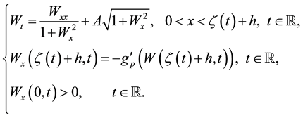
Lemma 4 Let ,
,  and
and . Assume that
 . Then
 (26)
(26)
where  is the average speed of the periodic traveling wave
  of (3)-(4) in band domain
 .
.
Proof From (7) we see that  satisfies

for all . So U is an upper solution of
 (27)
(27)
On the other hand, by Lemma 3  is a classical traveling wave of (27). So we can use comparison principle as in subsection 3.1 for
  and
and  on the interval
  to conclude that
 . ,
. ,
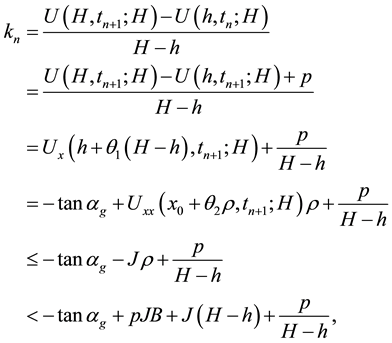
Proof of Main Theorem 3. We write g and  as
as  and
and , respectively. For any
 , since

we have


and

By Lemma 1 and the definitions of  and
and  we have
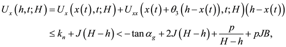
So  is a lower solution of
 (28)
(28)
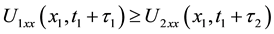
Replacing  in Lemma 3 by
 , respectively, we know that
is a classical traveling wave of (28). So we can use comparison principle for  and
and  in the interval
  to conclude that
On the other hand, replacing  by
by  in Lemma 4 we have
Combining the above inequalities with (25) we have

This proves Main Theorem 3). ,
4. Some Numerical Simulation Results
In this section we present some numerical simulation figures. Figure 2 indicates that the average speed c is strictly increasing in the basic width H of the domain.
Figure 3 indicates that the average speed c is strictly decreasing in the maximum opening angle .
.
Figure 4 indicates that the average speed c is strictly increasing in the period p of g.
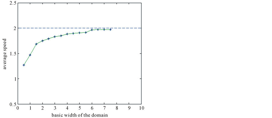
Figure 2. The monotonic dependence of c on H.
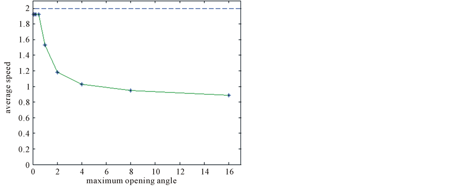
Figure 3. The monotonic dependence of c on α.
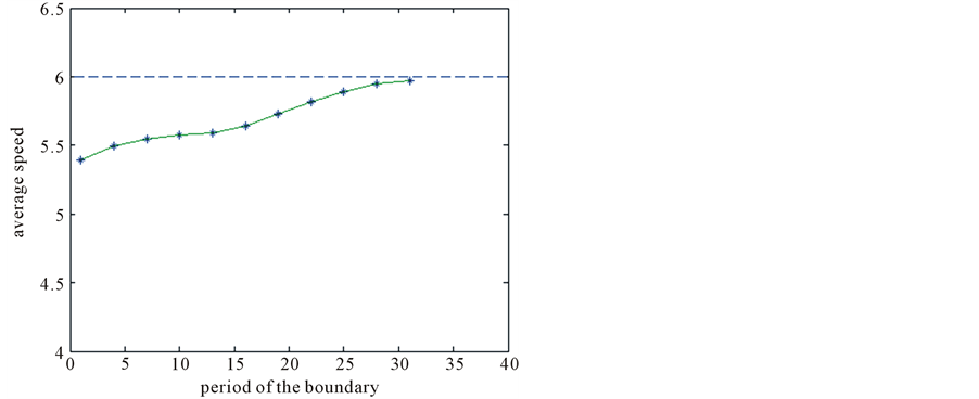
Figure 4. The monotonic dependence of c on p.
The results shown in Figure 2 and Figure 3 are partially proved in the main theorem. The dependence of c on p is very difficult, and we have no analytic result so far.
References
- Matano, H., Nakamura, K.I. and Lou, B. (2006) Periodic Traveling Waves in a Two-Dimensional Cylinder with Saw- Toothed Boundary and Their Homogenization Limit. Networks and Heterogeneous Media, 1, 537-568. http://dx.doi.org/10.3934/nhm.2006.1.537
- Alfaro, M., Hilhorst, D. and Matano, H. (2008) The Singular Limit of the Allen-Cahn Equation and the FitzHugh-Na- gumo System. Journal of Differential Equations, 245, 505-565. http://dx.doi.org/10.1016/j.jde.2008.01.014
- Lou, B. (2007) Singular Limits of Spatially Inhomogeneous Convection-Reaction-Diffusion Equation. Journal of Statistical Physics, 129, 509-516. http://dx.doi.org/10.1007/s10955-007-9400-3
- Nakamura, K.I., Matano, H., Hilhorst, D. and Schatzle, R. (1999) Singular Limits of Spatially Inhomogeneous Convection-Reaction-Diffusion Equation. Journal of Statistical Physics, 95, 1165-1185. http://dx.doi.org/10.1023/A:1004518904533
- Cioranescu, D. and Donato, P. (1999) An Introduction to Homogenization. Oxford University Press, Oxford.
- Cioranescu, D. and Saint Jean Paulin, J. (1999) Homogenization of Reticulated Structures. Springer-Verlag, New York.
- Protter, M.H. and Weinberger, H.F. (1967) Maximum Principles in Differential Equations. Prentice Hall, Englewood Cliffs, 172-173.