Optics and Photonics Journal, 2012, 2, 338-343
http://dx.doi.org/10.4236/opj.2012.24042 Published Online December 2012 (http://www.SciRP.org/journal/opj)
Speckle Reduction in Imaging Projection Systems
Weston Thomas, Christopher Middlebrook
Electrical and Computer Engineering Department, Michigan Technological University, Houghton, USA
Received October 10, 2012; revised November 15, 2012; accepted November 25, 2012
ABSTRACT
Diffractive diffusers (phase gratings) are routinely used for homogenizing and beam shaping for laser beam applications.
Another use for diffractive diffusers is in the reduction of speckle for pico-projection systems. While diffusers are un-
able to completely eliminate speckle they can be utilized to decrease the resultant contrast to provide a more visually
acceptable image. Research has been conducted to quantify and measure the diffusers overall ability in speckle reduc-
tion. A theoretical Fourier optics model is used to provide the diffuser’s stationary and in-motion performance in terms
of the resultant contrast level. Contrast measurements of two diffractive diffusers are calculated theoretically and com-
pared with experimental results. Having a working theoretical model to accurately predict the performance of the dif-
fractive diffuser allows for the verification of new diffuser designs specifically for pico-projection system applications.
Keywords: Diffractive Diffusers; Speckle Contrast Reduction; Laser Pico-Projectors
1. Introduction
The observance of speckle in laser images is caused by
the interference of the coherent source. Diffusers reduce
speckle by decreasing the temporal and spatial coherence
of the source. A diffuser has multiple cells each with
different phase values. By rotating or vibrating the dif-
fuser over a discrete time period the phase levels alter the
coherence, thereby reducing the speckle contrast. The
time-averaging of the speckle must occur over a discrete
time smaller than the integration time of the human eye.
Preceding investigations into the reduction of speckle
contrast using rotational diffusers are well known and
have had limited success [1-5]. The criterion for an ef-
fective diffuser is based on the calculation of the speckle
contrast. Equation (1) gives the contrast, calculated by
the standard deviation divided by the average intensity.

2
1
2
2
1
N
i
i
II
II N
CII





(1)
Figure 1 shows an example of a binary diffuser that is
currently being used for reducing speckle in laser projec-
tions systems and will be discussed in detail later. This
specific diffuser has circular symmetry for rotation pur-
poses.
2. Theory and Model
This diffuser is modeled as a single scattering phase
screen, written in the form of a transmission aperture,
given by Equation (2) [6]. Figure 2(a) illustrates the
placement of the diffuser in line with the initial beam and
followed by the imaging screen in the (x, y) plane which
has the varying phase pattern across the diffuser surface
as shown in Figure 3.

,
e
x
y
A
t

 (2)
The simulation will revolve around mimicking the op-
eration of two distinct diffuser types: binary and gray-
scale. The binary diffuser is based on a hadamard matrix
and thus contains only two distinct phase level sections.
This generates sharp edges in the output image. The
grayscale diffuser takes advantage of 64 discrete phase
levels creating a smoother granular profile [7]. Both
types are designed to reduce the visual degradation
Figure 1. Binary diffractive diffuser.
C
opyright © 2012 SciRes. OPJ

W. THOMAS, C. MIDDLEBROOK 339
(a) (b)
Figure 2. (a) Diffuser model layout; (b) Diffuser unit cell
layout.
(a)
(b)
Figure 3. (a) Grayscale diffuser array; (b) Binary diffuser
array.
caused by speckle through rotation. They are both mod-
eled with an array of 2000 × 2000 pixels. The phase
screen arrays are demonstrated in Figures 3(a) and (b).
Each diffuser is composed of individual cells replicated
across the surface as demonstrated in Figure 2(b). The
binary diffuser’s unit cell is an order 16 Hadamard ma-
trix while each Grayscale unit cell is a random organiza-
tion of the 64 phase levels. These two unit cells are ap-
proximations of the physical diffusers that were used for
experimental measurements but are not exact due to pro-
prietary information.
Equation (3) demonstrates the linear size limitation
given this array size and a z depth of 2 × 104 pixels.
Every individual phase element will consist of 25 pixels
for each diffuser model. The minimum phase element
size is 2.8 pixels for accurate sampling. This has been
increased to be arranged evenly and symmetrically across
the diffuser surface [8,9]. A distance mapping along the
optical axis can be characterized along the z-axis. Every
square pixel is related to a physical length by 2.5 µm.
This mapping can be established for the propagation axis,
z. This framing scale is maintained for all arrays unless
distinctly noted on the axis of the image.
z
xL

 (3)
For the discrete version, ∆x is the linear phase element
size, λ is the wavelength, z is the propagation distance in
pixels and L represents the total physical side length of
the array. The output from the aperture can be found by
using a Fourier approximation for distance propagation
such as the Fresnel equation [10]. Treating the mathe-
matical computation as a linear system allows the separa-
tion of code to flow freely with the functional partitions.
The system can be broken up into multiple parts as well
based on the needs of the simulation. In this instance it is
helpful to separate the Fourier optics propagation and the
diffuser rotational program from the individual diffuser
models allowing the diffuser models to be interchanged
without rewriting large amounts of the simulation.
The initial beam is considered to be a collimated
monochromatic Gaussian beam, as demonstrated in Fig-
ure 4, which is defined as [11]

 
22
2
0
,e
ab
w
G
U


 

 

 

 (4)
where the position (a, b) is the center of the Gaussian
beam, is the beam waist, and

,


  represents the
physical size divided by the number of pixels in each
direction. The laser wave front will be the size reference
from which the rest of the simulation is measured. The
xy-plane is the plane of incidence of the wave-front. The
Gaussian beam is propagated through the diffuser in two
steps. First the wave is multiplied by the transmission
aperture, A adding a phase displacement to the initial
beam. The output of this calculation, shown in Equation
(5), represents the field directly after the diffuser [12].
t

W. THOMAS, C. MIDDLEBROOK 340
Figure 4. Gaussian beam profile.
(a)
(b)
Figure 5. (a) Stationary binary diffuser; (b) Stationary
grayscale diffuser.


1,, G
UU   A t (5)
The second part involves the Fourier propagation of
onto the (x, y) image plane. This is accomplished through
the Fresnel approximation of the Rayleigh-Sommerfield
equation [8,13]. The Fresnel approximationis given in
Equation (6) where

is the wavelength, is the
wavenumber, is the propagation distance along the
optical axis and
k
z


,

 is the aperture plane. The
wavelength, once again, is chosen to be 535 nm, repre-
senting a generic green laser diode as well as the center
wavelength of the visible spectrum.
 

22
2
2
1
e
,,e
k
jkz jx y
z
UxyU
jz

dd







  (6)
The final field image cannot be generated too close to
the diffuser without causing quadratic errors in the ex-
ponential component. Using previous values for the dif-
fuser aperture size and imaging array size, 1600 and
2000 pixels respectively, a proximity limit of 4500 pixels
is calculated using Equation (7). This is considered the
near-field region of measurement [13]. While the Fresnel
integral does work in the far-field, the loss of image clar-
ity due to beam expansion makes it less convenient to
use and the model will refrain from approaching that
region, defined by Equation (8) [13].

2
22
3
max
π
4
zxy 






 (7)


2
22
max
2
k
z
 
 (8)
The final section of the simulation involves the rota-
tion of the diffuser and the modeling of a camera or cap-
ture device. Using previous data, the diffuser can be suf-
ficiently operated at 60 (+/−0.5) revolutions per second
[3]. In addition, the camera will operate at 30 Hz, to
mimic the eye’s refresh rate or sampling time of around
23 frames per second [14]. To accomplish this the dif-
fuser array will be rotated prior to propagation of the
field


1,U

 . The formation of the final image is com-
pleted by addition of the individual fields while main-
taining pixel position


,jk as characterized by Equa-
tion (9).
The final field is then normalized by the total number
of images, h. The intensity image is then found by
squaring the absolute value of the field,


,
F
Uxy
. A
capture device integrates on the order of 1020 photons for
a single image during a predetermined exposure time. In
order to represent this, an approximation is resolved.
This was completed through a series of Monte Carlo
simulations. A generic noise pattern was created and then
rotated a single revolution. The images were rotated and
integrated at various degree increments ranging from

W. THOMAS, C. MIDDLEBROOK 341
0.01 degrees to 60 degrees. The resolution of the various
images was compared against one another until the indi-
vidual noise parameters were indistinguishable. This is
the degree resolution from which the simulation will be
completed. With the degree resolution defined at 0.75 the
total number of images integrated to create a single frame
is 480. Comparing the speed of the diffuser at 60 Hz to
the camera integration speed of 30 Hz it is identified that
2 rotations are completed for every single image frame.
This will require at least 144,000 distinct images to rep-
resent a 10 second video capture.
3. Results
Calculations were made for the speckle contrast of sta-
tionary and moving diffuser images using Equation (1).
The images for the stationary diffusers are shown below
in Figures 5(a) and (b) for the binary and grayscale ver-
sions, respectively. The central spot of the diffuser is the
zero-order diffractive mode. Most diffractive optical ele-
ments will consist of some form of zero-order mode and
is considered to be the DC portion of the element. An
optimum diffuser will minimize this zero-order and
smooth out the overall output profile of the speckle. The
first order of the element contains the majority of the
incident power, 90% (+/−5%) as measured experimen-
tally, as well as the highest speckle reductive properties.
The speckle contrast is calculated for this first order spot
of the diffuser image. The binary version has a contrast
of 0.76 and the grayscale version has a contrast value of
0.74. These values correspond to data taken from inten-
sity images of the simulation.
Close up versions of the central order of the diffuser
image are shown in Figures 6(a) and (b). This is the
physical representation of a focused image from the dif-
fuser. They are 300 × 300 pixel array snapshots of the
total diffuser image from above. This can be directly
compared with bench top experiments taken using binary
and grayscale diffusers with a 532 nm DPSS laser [3].
The camera used for the physical experiments had a 480
× 640 pixel array. The stationary, focused diffuser im-
ages are shown in Figures 6(c) and (d). The contrast
values for the bench top experiment are 0.77 for the bi-
nary diffuser and 0.68 for the grayscale version. The
contrast values themselves are accurate to within 10%.
The images themselves, however, are not as comparable.
The simulated versions have a more rigid structure while
the bench top images are more fluid and organic, spe-
cifically related to the binary diffuser image. It is be-
lieved that this is a result of the inputs for the creation of
the individual diffusers. The contrast results alone do
provide enough accuracy for the simulation to be ac-
ceptable.
The simulation is finished by creating rotating varia-
tions of the diffuser patterns and propagating them onto
(a) (b)
(c) (d)
Figure 6. (a) Focused, stationary binary diffuser; (b) Fo-
cused, stationary grayscale diffuser; (c) Physical binary
diffuser output intensity image; (d) Physical grayscale dif-
fuser output intensity image.
the image plane. The parameters were set to mimic the
rotational speed of the diffser as 60 Hz. The speckle
was only mas for the
stationary diffuser images. The simulated images are
slightly less at 0.18 for the
As mentioned earlier, the diffusers were illuminated
u
easured for the central order as it w
shown in Figures 7(a) and (b). The calculated contrast
values for the binary and grayscale images are 0.297 and
0.276, respectively. The contrast values found in the
ench top experiments wereb
binary and 0.14 for the grayscale versions. This relates to
a contrast difference of around 10% - 13% contrast re-
duction between simulation and actual results.
The current version of this model focuses on a singles-
cattering approach [4]. While this approach provides a
close approximation it does not fully agree with the
physical diffuser scattering profile. This will be the main
concentration for future work with the project. It is also
assumed that a single polarization is incident on the dif-
fusers and that the diffusers are polarization maintaining.
Previous research showed that the polarization incident
on the diffuser did not have an impact on the final con-
trast results [3]. This is an approximation that can be
changed in the simulation to ensure the theoretical and
experimental results match up. The simulation is still a
good approximation as it does keep the contrast reduc-
tion rate between stationary and rotational the same at
around 50% speckle decrease. This allows the simulation
to become a useful tool for preliminary design work with
theoretical diffuser shapes.

W. THOMAS, C. MIDDLEBROOK 342
(a)
(b)
Figure 7. (a) Stationary binary diffuser; (b) Stationary
grayscale diffuser.
with a coherent Gaussian source. All contrast values
were measured without subtracting the Gaussian beam
difference in the speckle. While uniform illumination
speckle statistics are generally considered proper, it is by
no means correct as standard laser diodes will have som
sort of Gaussian shell and speckle created from such
on model and comparisons were made between uniform
e
any
a diode will have statistics correlating to the Gaussian
laser beam. Verification was completed using the simula-
ti
illumination and a Gaussian source. Minor differences
can be seen within Figure 6 but the primary result of the
Gaussian illumination is the slight spreading of the
speckle pattern and lower intensity within the center.
Based on the speckle numbers this result is trivial and
evens out across the final image plane, as demonstrated
through Figures 8(a) and (b).
4. RGB Integration
In order to make full use of this model for a projector
system more than one color must be combined for an
(a) (b)
Figure 8. (a) Diffuser model with uniform illumination; (b)
Diffuser model with Gaussian illumination.
image. Most diffusers are created for a single wavelength
and errors result from using polychromatic light or mul-
tiple wavelengths. This problem will need to be solved
before full implementation of diffusers into pico-projec-
tors can be accomplished. In addition, integration of mul
tiple colors in its own
th diffusers.
-
to a single image can be difficult on
due to the variation in the human eye’s perception of
colors [15]. Simulation will help to reduce problems in
e creation and testing of multi-wavelength
Beginning experiments were conducted to measure the
wavelength dependence of the diffuser designs. The dif-
fuser arrays were tested at wavelengths 635 and 450 nm
to compare with the 535 nm beam results. The three
wavelengths individual images for the grayscale diffuser
simulation are shown in Figures 9(a)-(c). All three
wavelength simulations were completed at the same dis-
tance from the diffuser along the optical axis. The obvi-
ous comparison between them is the expansion of the
overall wave front. Speckle contrast measurements were
taken for the central order of the diffuser. The contrast
for the 450 nm image is 0.711 and is 0.65 for the 635 nm
image.
The simulated images also allow the ability to com-
bine the three wavelengths together into a single RGB
image. Figure 9(d) illustrates this process and shows
how the three distinct grayscale speckle patterns overlay
onto one another. Current speckle calculations do not
allow for 3 dimensional measurements and thus any cal-
culation would simply be an average of the results for
reach individual wavelength. In this case such an average
gives a speckle contrast of 0.70 for the simulated gray-
scale diffuser. Also the colored images had to be nor-
malized based on the visual response of the eye. Other-
wise, the colors would appear out of sync and any
speckle measurements would not align with visual rep-
resentation of the speckle image [16]. A new measure-
ment protocol will be needed to fully realize the speckle
reduction ability of a diffuser design. Current investiga-
tions have led to comparisons between correlation times
of diffusers and their resultant speckle contrast.

W. THOMAS, C. MIDDLEBROOK 343
(a) (b)
(c) (d)
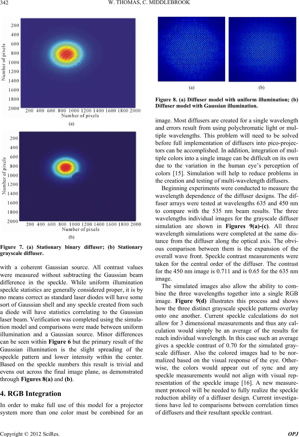
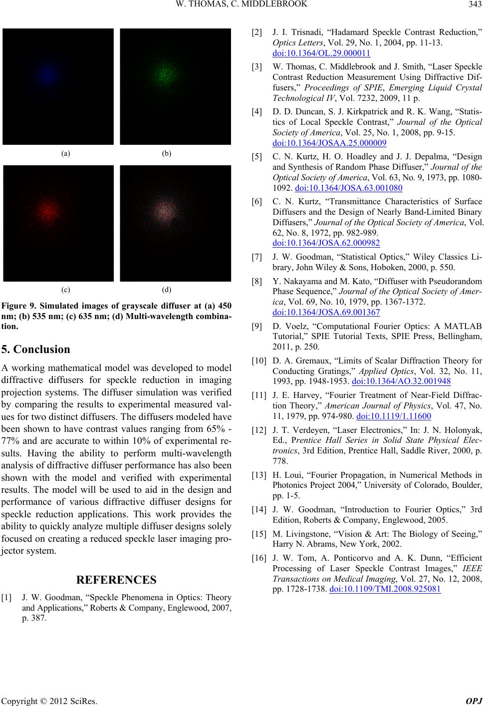
Figure 9. Simulated images of grayscale diffuser at (a)
nm; (b) 535 nm; (c) 635 nm; (d) Multi-wavelength combina-
tion.
5. Conclusion
A working mathematical model was developed to model
diffractive diffusers for sle reduction in imaging
projection syst was ve
by comparing the results to experimental measured val-
ues for two distinct diffusers. The diffusers modeled have
been shown to have contrast values ranging from 65% -
77% and are accurate to within 10% of experiment
sults. Having the ability to perform multi-waveleng
analysis of diffractive diffuser performance has also been
shown with the model and verified with experim
results. The model will be used to aid in the design and
performance of various diffractive diffuser designs for
speckle reduction applicatins. This work provides th
ability to quickns so
REFERENCES
450
peck
ems. The diffuser simulationrified
al re-
th
ental
o e
lely analyze multiple diffuser desigly
focused on creating a reduced speckle laser imaging pro-
jector system.
[1] J. W. Goodman, “Speckle Phenomena in Optics: Theory
and Applications,” Roberts & Company, Englewood, 2007,
p. 387.
[2] J. I. Trisnadi, “Hadamard Speckle Contrast Reduction,”
Optics Letters, Vol. 29, No. 1, 2004, pp. 11-13.
doi:10.1364/OL.29.000011
[3] W. Thomas, C. Middlebrook and J. Smith, “Laser Speckle
Contrast Reduction Measurement Using Diffractive Dif-
fusers,” Proceedings of SPIE, Emerging Liquid Crystal
Technological IV, Vol. 7232, 2009, 11 p.
[4] D. D. Duncan, S. J. Kirkpatrick and R. K. Wang, “Statis-
tics of Local Speckle Contrast,” Journal of the Optical
Society of America, Vol. 25, No. 1, 2008, pp. 9-15.
doi:10.1364/JOSAA.25.000009
[5] C. N. Kurtz, H. O. Hoadley and J. J. Depalma, “Design
and Synthesis er,” Journal of the
Optical Society. 9, 1973, pp. 1080-
of Random Phase Diffus
of America, Vol. 63, No
1092. doi:10.1364/JOSA.63.001080
[6] C. N. Kurtz, “Transmittance Characteristics of Surface
Diffusers and the Design of Nearly Band-Limited Binary
Diffusers,” Journal of the Optical Society of America, Vol.
62, No. 8, 1972, pp. 982-989.
doi:10.1364/JOSA.62.000982
[7] J. W. Goodman, “Statistical Optics,” Wiley Classics Li-
brary, John Wiley & Sons, Hoboken, 2000, p. 550.
[8] Y. Nakayama and M. Kato, “Diffuser with Pseudorandom
Phase Sequence,” Journal of the Optical Society of Amer-
ica, Vol. 69, No. 10, 1979, pp. 1367-1372.
doi:10.1364/JOSA.69.001367
[9] D. Voelz, “Computational Fourier Optics: A MAT
Tutorial,” SPIE Tutorial Texts,
LAB
SPIE Press, Bellingham,
.32.001948
2011, p. 250.
[10] D. A. Gremaux, “Limits of Scalar Diffraction Theory for
Conducting Gratings,” Applied Optics, Vol. 32, No. 11,
1993, pp. 1948-1953. doi:10.1364/AO
[11] J. E. Harvey, “Fourier Treatment of Near-Field Diffrac-
tion Theory,” American Journal of Physics, Vol. 47, No.
11, 1979, pp. 974-980. doi:10.1119/1.11600
[12] J. T. Verdeyen, “Laser Electro
Ed., Prentice Hall Series in S
nics,” In: J. N. Holonyak,
olid State Physical Elec-
n to Fourier Optics,” 3rd
ms, New York, 2002.
, 2008,
tronics, 3rd Edition, Prentice Hall, Saddle River, 2000, p.
778.
[13] H. Loui, “Fourier Propagation, in Numerical Methods in
Photonics Project 2004,” University of Colorado, Boulder,
pp. 1-5.
[14] J. W. Goodman, “Introductio
Edition, Roberts & Company, Englewood, 2005.
[15] M. Livingstone, “Vision & Art: The Biology of Seeing,”
Harry N. Abra
[16] J. W. Tom, A. Ponticorvo and A. K. Dunn, “Efficient
Processing of Laser Speckle Contrast Images,” IEEE
Transactions on Medical Imaging, Vol. 27, No. 12
pp. 1728-1738. doi:10.1109/TMI.2008.925081