Paper Menu >>
Journal Menu >>
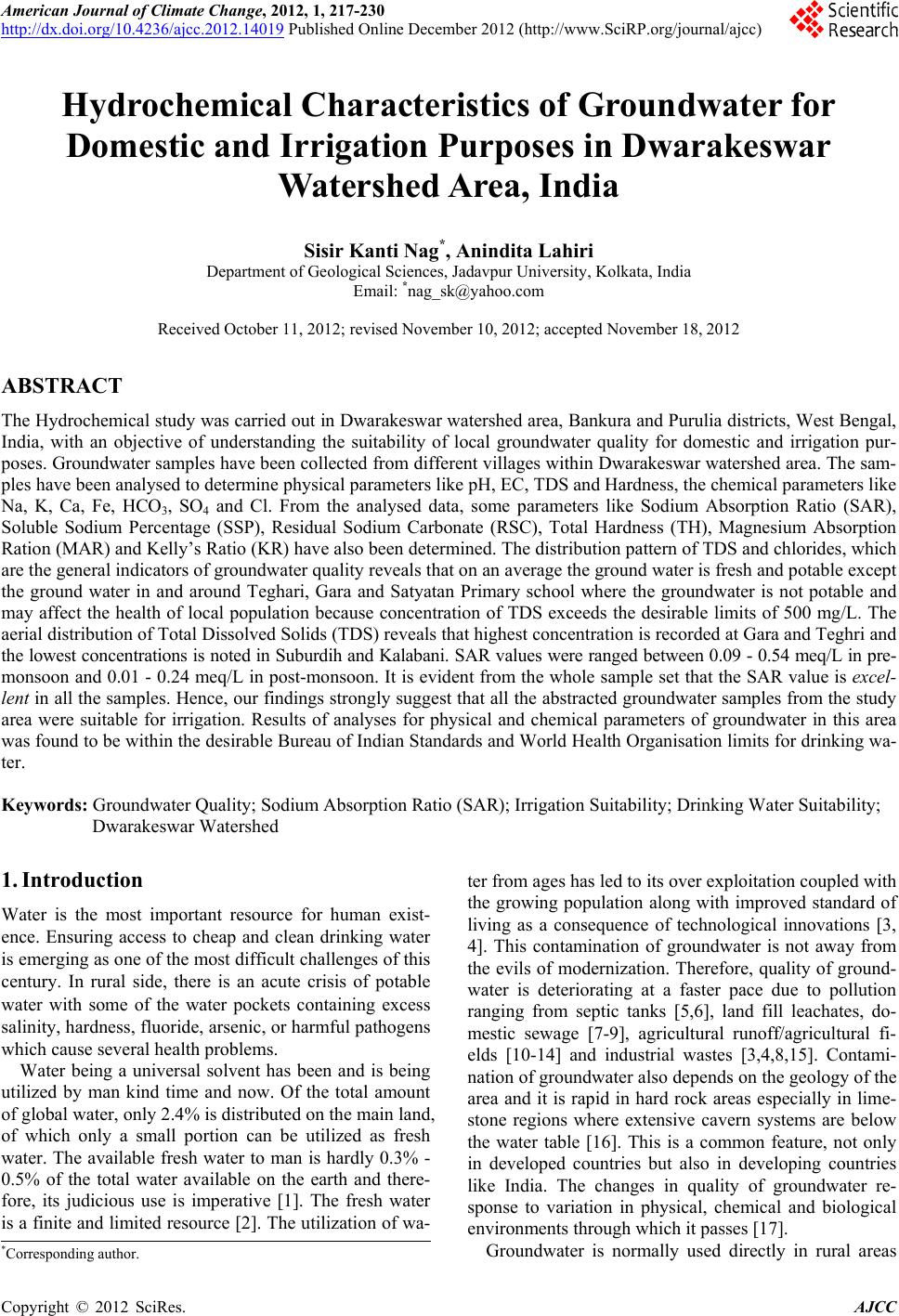 American Journal of Climate Change, 2012, 1, 217-230 http://dx.doi.org/10.4236/ajcc.2012.14019 Published Online December 2012 (http://www.SciRP.org/journal/ajcc) Hydrochemical Characteristics of Groundwater for Domestic and Irrigation Purposes in Dwarakeswar W atershed Area, India Sisir Kanti Nag*, Anindita Lahiri Department of Geological Sciences, Jadavpur University, Kolkata, India Email: *nag_sk@yahoo.com Received October 11, 2012; revised November 10, 2012; accepted November 18, 2012 ABSTRACT The Hydrochemical study was carried out in Dwarakeswar watershed area, Bankura and Purulia districts, West Bengal, India, with an objective of understanding the suitability of local groundwater quality for domestic and irrigation pur- poses. Groundwater samples have been collected from different villages within Dwarakeswar watershed area. The sam- ples have been analysed to determine physical parameters like pH, EC, TDS and Hardness, the chemical parameters like Na, K, Ca, Fe, HCO3, SO4 and Cl. From the analysed data, some parameters like Sodium Absorption Ratio (SAR), Soluble Sodium Percentage (SSP), Residual Sodium Carbonate (RSC), Total Hardness (TH), Magnesium Absorption Ration (MAR) and Kelly’s Ratio (KR) have also been determined. The distribution pattern of TDS and chlorides, which are the general indicators of groundwater quality reveals that on an average the ground water is fresh and potable except the ground water in and around Teghari, Gara and Satyatan Primary school where the groundwater is not potable and may affect the health of local population because concentration of TDS exceeds the desirable limits of 500 mg/L. The aerial distribution of Total Dissolved Solids (TDS) reveals that highest concentration is recorded at Gara and Teghri and the lowest concentrations is noted in Suburdih and Kalabani. SAR values were ranged between 0.09 - 0.54 meq/L in pre- monsoon and 0.01 - 0.24 meq/L in post-monsoon. It is evident from the whole sample set that the SAR value is excel- lent in all the samples. Hence, our findings strongly suggest that all the abstracted groundwater samples from the study area were suitable for irrigation. Results of analyses for physical and chemical parameters of groundwater in this area was found to be within the desirable Bureau of Indian Standards and World Health Organisation limits for drinking wa- ter. Keywords: Groundwater Quality; Sodium Absorption Ratio (SAR); Irrigation Suitability; Drinking Water Suitability; Dwarakeswar Watershed 1. Introduction Water is the most important resource for human exist- ence. Ensuring access to cheap and clean drinking water is emerging as one of the most difficult challenges of this century. In rural side, there is an acute crisis of potable water with some of the water pockets containing excess salinity, hardness, fluoride, arsenic, or harmful pathogens which cause several health problems. Water being a universal solvent has been and is being utilized by man kind time and now. Of the total amount of global water, only 2.4% is distributed on the main land, of which only a small portion can be utilized as fresh water. The available fresh water to man is hardly 0.3% - 0.5% of the total water available on the earth and there- fore, its judicious use is imperative [1]. The fresh water is a finite and limited resource [2]. The utilization of wa- ter from ages has led to its over exploitation coupled with the growing population along with improved standard of living as a consequence of technological innovations [3, 4]. This contamination of groundwater is not away from the evils of modernization. Therefore, quality of ground- water is deteriorating at a faster pace due to pollution ranging from septic tanks [5,6], land fill leachates, do- mestic sewage [7-9], agricultural runoff/agricultural fi- elds [10-14] and industrial wastes [3,4,8,15]. Contami- nation of groundwater also depends on the geology of the area and it is rapid in hard rock areas especially in lime- stone regions where extensive cavern systems are below the water table [16]. This is a common feature, not only in developed countries but also in developing countries like India. The changes in quality of groundwater re- sponse to variation in physical, chemical and biological environments through which it passes [17]. Groundwater is normally used directly in rural areas *Corresponding author. C opyright © 2012 SciRes. AJCC 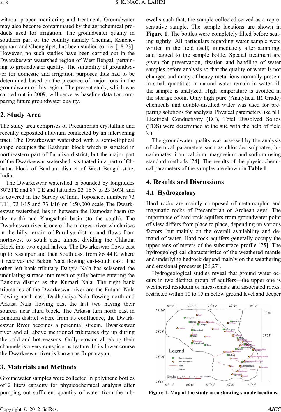 S. K. NAG, A. LAHIRI 218 without proper monitoring and treatment. Groundwater may also become contaminated by the agrochemical pro- ducts used for irrigation. The groundwater quality in southern part of the country namely Chennai, Kanche- epuram and Chengalpet, has been studied earlier [18-23]. However, no such studies have been carried out in the Dwarakeswar watershed region of West Bengal, pertain- ing to groundwater quality. The suitability of groundwa- ter for domestic and irrigation purposes thus had to be determined based on the presence of major ions in the groundwater of this region. The present study, which was carried out in 2009, will serve as baseline data for com- paring future groundwater quality. 2. Study Area The study area comprises of Precambrian crystalline and recently deposited alluvium connected by an intervening tract. The Dwarkeswar watershed with a semi-elliptical shape occupies the Kashipur block which is situated in northeastern part of Puruliya district, but the major part of the Dwarkeswar watershed is situated in a part of Ch- hatna block of Bankura district of West Bengal state, India. The Dwarkeswar watershed is bounded by longitudes 86˚51'E and 87˚0'E and latitudes 23˚16'N to 23˚50'N. and is covered in the Survey of India Toposheet numbers 73 I/11, 73 I/15 and 73 I/16 on 1:50,000 scale The Dwark- eswar watershed lies in between the Damodar basin (to the north) and Kangsabati basin (to the south). The Dwarkeswar river is one of them largest river which rises in the hilly terrain of Puruliya district and flows from northwest to south east, almost dividing the Chhatna Block into two equal halves. The Dwarkeswar flows east up to Kashipur and then South east from 86˚44'E. where it receives the Bekon Nala flowing east-south east. The other left bank tributary Dangra Nala has scissored the undulating surface into mesh of gully before entering the Bankura district as the Kumari Nala. The right bank tributaries of the Dwarkeswar river are the Futuari Nala flowing north east, Dudhbhaiya Nala flowing north and Arkasa Nala flowing east the last two having their sources near Hura block. The Arkasa turn north east in Bankura district where from its confluence, the Dwark- eswar River becomes a perennial stream. Dwarkeswar river and all above mentioned tributaries dry up during the cold and hot seasons. Gully erosion all along their channels is a very conspicuous feature. In its lower course the Dwarkeswar river is known as Rupnarayan. 3. Materials and Methods Groundwater samples were collected in polythene bottles of 2 liters capacity for physicochemical analysis after pumping out sufficient quantity of water from the tub- ewells such that, the sample collected served as a repre- sentative sample. The sample locations are shown in Figure 1. The bottles were completely filled before seal- ing tightly. All particulars regarding water sample were written in the field itself, immediately after sampling, and tagged to the sample bottle. Special treatment are given for preservation, fixation and handling of water samples before analysis so that the quality of water is not changed and many of heavy metal ions normally present in small quantities in natural water remain in water till the sample is analyzed. High temperature is avoided in the storage room. Only high pure (Analytical IR Grade) chemicals and double-distilled water was used for pre- paring solutions for analysis. Physical parameters like pH, Electrical Conductivity (EC), Total Dissolved Solids (TDS) were determined at the site with the help of field kit. The groundwater quality was assessed by the analysis of chemical parameters such as chlorides sulphates, bi- carbonates, iron, calcium, magnesium and sodium using standard methods [24]. The results of the physicochemi- cal parameters of the samples are shown in Table 1. 4. Results and Discussions 4.1. Hydrogeology Hard rocks are mainly composed of metamorphic and magmatic rocks of Precambrian or Archean ages. The importance of hard rock aquifers from groundwater point of view differs from place to place, depending on various factors, but mainly on the overall availability and de- mand of water. Hard rock aquifers generally occupy the upper tens of meters of the subsurface profile [25]. The hydrogeologi cal characteristics of the weathered mantle and underlying bedrock depend mainly on the weathering and erosional processes [26,27]. Hydrogeological studies reveal that ground water oc- curs in two distinct group of aquifers—the upper one is weathered residuum of mica-schists and associated rocks, restricted within 10 to 15 m below ground level and deeper Figure 1. Map of the study area showing sample locations. Copyright © 2012 SciRes. AJCC  S. K. NAG, A. LAHIRI Copyright © 2012 SciRes. AJCC 219 Table 1. Report of physico-chemical parameters of the studied groundwater samples (pre-monsoon and post-monsoon, 2009). Chemical Parameters Physical Parameters Anions Cations pH EC (S/cm) TDS (mg/L) Hardness (mg/L) Cl (mg/L) HCO3 (mg/L) SO4 (mg/L) Fe (mg/L) Mg (mg/L) Ca (mg/L) Na (mg/L) Sample No. Location Name prepost prepostpre p os t pre postpr e post pre postpre postprepostprepostprepostprepost A1 Dubrajpur More 7.97.1340 700218257210 230706026022076.134.10.800.254.322.0722.7430.067.531.27 A2 Satyatan p.school 7.77.1190300122122100130404011017047.576.30.500.8 3.924.83 9.9859.946.375.21 A3 D warkeswa r R. Bed 7.96.4180400115 122901070 203011017012.242.9 0.10 0.44.204.1814.4046.436.573.72 A4 Teghri 6.76.6185 0 3400118413651030750640580 180 28053.776.40.500.85.204.7153.74113.2411.474.16 A5 Gara 7.06.5194 0 24001242948119020066034021031024.4127.30.301.35.163.1252.55 98.53 11.572.03 A6 Suburdih6.46.513030083130903304011013019041.6116.50.501.23.343.516.3979.965.354.07 A7 Kamalpur7.07.04809003073342802003040430350127.8138.43.003.04.813.7121.6140.066.994.59 A8 Sukhnibash6.16.445090028833320031090110140150153.143.53.000.54.393.6218.1936.5310.017.83 A9 Jhatipahari6.16.459040037832735021011010015023098.521.63.000.24.873.7824.0230.078.106.87 A10Morgaboni6.36.5220 500141177140 210 2050160 23026.325.90.300.24.213.67 12.4184.576.575.71 A11Kharbona7.56.65901300378495400 42080110 780 35037.228.50.300.34.714.1330.8459.969.347.52 A12Narandihi7.27.1460 800294360240 2707050240 25086.727.40.800.24.693.4123.6974.866.616.32 A13 Kanudi 6.56.5170300109104901501040130180152.431.51.200.34.324.818.0979.535.237.26 A14Bhagbanpur7.17.1220 400141144110 2002020120 17023.627.50.302.04.244.8310.68103.275.225.02 A15Hutgram6.67.1220 400141153100 140103016021047.936.90.503.04.804.889.64214.236.507.53 A16 Chaitor 6.96.9780110049944246043016012025029042.211.60.500.34.813.7944.2943.766.996.52 A17 Goaldanga7.46.48801500563542460 450220200 160 17059.424.70.500.34.853.9241.0636.298.655.74 A18Kalabani6.6 6.83502001340921010190570 3029018073.635.70.700.14.962.07110.6 4 43.873.94 1.04 A19Damankiari6.46.6130900438325380 3309090140 21036.339.60.3033.763.5236.4273.653.583.68 A20 Simla 6.86.4120160044763347046012731031023043.128.50.401.24.132.1646.7368.273.975.83 A21Kashipur6.66.2160 800540283490 260220110 190 18016.3.321.60.201.24.762.2338.7953.948.374.39 A22 Rugri 6.66.92101700115462298266036025035033056.824.730.761.22.862.3894.6857.735.276.84 A23Kapistha 6.56.9280 2003094160 12031030320 140112.720.050.800.13.721.9379.3753.263.946.38 A24 Bhatin 6.96.6207150037657438550017017034021036.322.730.301.23.842.3458.6941.375.824.72 A25 Sutabai 6.76.6210180017472148050014025028018018.717.630.300.54.863.26114.3 7 68.385.86 5.96 A26 Natungram7.2 6.850 900363531402206290130280163.946.382.070.44.873.1778.4161.946.483.46 A27Sialdanga 7.16.440 2500148100 8 130 80068400 130 39018329.72.040.24.962.0678.4152.176.485.29 one represented by fractures occurring at varying depth between 30 m to 150 m below ground level. Both the aquifers are the repositories of ground water within sec- ondary porosities developed due to geological process. The first aquifers is developed by due wells and solely used for drinking and other domestic purposes. The sec- ond aquifer (fracture zones) being exploited for industrial water supply are also used for drinking water supply. Ground water is hidden from view beneath the land surface, it can only be directly observed through moni- toring wells. In order to assess water level configuration of different aquifers, hydrogeological studies have been carried out. The upper aquifer is tapped by open dug wells and mainly used for domestic consumption. Bore  S. K. NAG, A. LAHIRI 220 wells in different industries withdrawal water from the deeper fracture zones, which occurs under semi-confined to confined conditions. Altogether 27 nos. of bore wells and 24 nos. of dug wells were marked and monitored for having an idea of water table in pre- and post-monsoon 2009 (Figure 2). Water table studies indicate that groundwater level varies in between 95.94 mts to 193.17 mts. in pre-monsoon. Highest value of water table is recorded in Damankiari area. In post-monsoon water table studies indicate that groundwater level varies in between 98.41 m to 195.70 m. Highest value of water table is recorded in Kalabani area (Figures 2 (a) and (b)). In case of dug well water table varies between 105.05 mts to 193.88 mts in pre-monsoon and in post-monsoon it varies between 108.25 mts to 196.88 mts. Lowest value of water table is recorded in Hanuliya area 105.5 mts and 108.25 mts during pre-and post-monsoon respectively. Water table contour map of dug well indicates the for- (a) (b) Figure 2. Water table contour map of the study area bore well: (a) pre-monsoon; (b) post-monsoon. mation of a cone of depression in the area surrounding Teghori and Jambani in pre- and post-monsoon time (Figures 3 (a) and (b)) 4.2. Major Ion Chemistry and Spatial Distribution The pH values of the groundwater varied from 6.1 to 7.9 with an average value 6.9 (pre-monsoon) while the pH values range between 6.2 to 7.1 (post-monsoon) with an average value 6.7. This indicates that water is neutral in nature. The variation in pH values both in pre- and post- monsoon periods are shown in Fi gures 4(a) and (b). In the study area, the value of electrical conductivity varied from 40 - 1940 μS/cm with an average value of 423.96 μS/cm during pre-monsoon while the value rang- ed between 200 - 3400 μS/cm with an average of 1040.74 μS/cm during post-monsoon period (Figures 5(a) and (b)). In the study area, the concentration value of TDS 86.55 86.6 86.65 86.7 86.75 86.8 86.85 86.9 86.9587 23.2 23.25 23.3 23.35 23.4 23.45 23.5 kashipur simla Damankiari Kalabani sonaijuri Rudra sialdanga Balarampur Hanulia Dalpur Murgabani Arra Dubrajpur Jhagrapur Bijpur Kamalpur Bahara Teghori Kendsaer Jambani Danmari Bhimpur Niasa Kelai 105110115120125130135140145150155160165170175180185190195 Contour Scale (a) 86.55 86.6 86.65 86.7 86.75 86.8 86.85 86.9 86.9587 23.2 23.25 23.3 23.35 23.4 23.45 23.5 kashipur simla Damankiari Kalabani sonaijuri Rudra sialdanga Balarampur Hanulia Dalpur Murgabani Arra Dubrajpur Jhagrapur Bijpur Kamalpur Bahara Teghori Kendsaer Jambani Danmari Bhimpur Niasa Kelai 105110115120125130135140145150155160165170175180185190195 Contour Scale (b) Figure 3. Water table contour map of the study area dug well: (a) pre-monsoon; (b) post-monsoon. Copyright © 2012 SciRes. AJCC  S. K. NAG, A. LAHIRI 221 ranged between 30 to 1340 mg/L (pre-monsoon) with the mean value of 403.18 mg/L. The TDS value ranged be- tween 92 to 1365 mg/L (post-monsoon) with the mean value of 409.63 mg/L. The TDS of the study area falls within the WHO (2004) Standard of 1000 mg/L. The wa- ter is thus good for human consumption (domestic) and agricultural purposes (Figures 6(a) and (b)). The total hardness expressed as CaCO3 is above the desirable limit (300 mg/L) and allowable limit is (600 mg/L). The hardness is temporary in nature and can be removed by boiling. The water samples of the study area show variation from 90 - 1190 mg/L (pre-monsoon) with an average value of 376.55 mg/L while the value of hardness ranged between 120 - 1070 mg/L during post- monsoon period with the average value of 360.74 mg/L (Figures 7 (a) and (b)) The hardness in water is derived from the solution of carbon dioxide released by bacterial action in the soil, in percolating rain water. Low pH conditions develop and lead to the dissolution of insoluble carbonates in the soil and in limestone formations to convert them into soluble 86.55 86.6 86.65 86.7 86.75 86.8 86.85 86.9 86.9587 23.2 23.25 23.3 23.35 23.4 23.45 23.5 66.16.26.36.46.56.66.76.86.977.17.27.37.47.57.67.77.87.98 Contour Scale (a) 86.55 86.6 86.65 86.7 86.75 86.8 86.85 86.9 86.9587 23.2 23.25 23.3 23.35 23.4 23.45 23.5 55.25.45.65.866.26.46.66.877.27.47.67.88 Contour Scale (b) Figure 4. pH contour map: (a) pre-monsoon; (b) post-mon- soon. bicarbonates. Impurities in limestone, such as sulfates, chlorides and silicates, become exposed to the solvent action of water as the carbonates are dissolved so that they also pass into solution. The general acceptance level of hardness is 300 mg/L, although WHO [23] has set an allowable limit of 600 mg/L. The spatial distribution pat- tern of physical parameters like pH, Electrical Conduc- tivity (EC), Total Dissolved Solids (TDS) during the study period are shown in Figures 4(a) and (b), Figures 5(a) and (b) and Figures 6(a) and (b). In the study area, the concentration of chloride is found to vary between 10 - 660 mg/L with the average value of 163.2 mg/L in pre-monsoon while during post- monsoon the value ranged between 20 - 580 mg/L with the mean value of 139.3 mg/L (Figures 8(a) and (b)). The mean values during pre- and post-monsoon time are much below the maximum allowable concentration of 250 mg/L [28]. WHO has set standards of 200 - 500 mg/L for chloride in drinking water. Too much of chloride leads to bad taste in water and also chloride ion combines with the Na (that is being derived from the weathering of (a) 86.55 86.686.6586.7 86.7586.8 86.85 86.986.9587 23.2 23.25 23.3 23.35 23.4 23.45 23.5 00.511.522.533.5 Contour Scale (b) Figure 5. Specific conductivity contour map: (a) pre-mon- soon; (b) post-monsoon. Copyright © 2012 SciRes. AJCC  S. K. NAG, A. LAHIRI 222 86.6 86.65 86.7 86.75 86.8 86.85 86.9 86.95 23.2 23.25 23.3 23.35 23.4 23.45 301302303304305306307308309301030113012301330 Contour Scale (a) 86.55 86.6 86.65 86.7 86.75 86.8 86.85 86.9 86.9587 23.2 23.25 23.3 23.35 23.4 23.45 23.5 0200400600800100012001400 Contour Scale (b) Figure 6. Total dissolved solids contour map: (a) pre-mon- soon; (b) post-monsoon. granitic terrains) and forms NaCl, whose excess presence in water makes it saline and unfit for drinking and irriga- tion purposes. Here too, as exhibited by contours, the chloride value decreases during post-monsoon. Bicarbonate ion varied from 110 to 780 and with mean value of 229.6 mg/L during pre-monsoon and 140 to 390 mg/L with average value of 231.5 mg/L in the ground- water samples of post-monsoon season period (Figures 9(a) and (b)). The sulfate ion causes no particular harmful effects on soils or plants; however, it contributes to increase the salinity in the soil solution. Sulphur is an essential ele- ment in plant nutrition and in the form of sulphate it is readily available to plants. Sulfate ion varied from 12.2 to 183.0 mg/L during the pre-monsoon and from 11.6 to 138.4 mg/L in post-monsoon seasons (Figures 10(a) and (b)). Calcium and magnesium ions present in groundwater (a) 86.55 86.6 86.65 86.7 86.75 86.8 86.85 86.986.9587 23.2 23.25 23.3 23.35 23.4 23.45 23.5 01002003004005006007008009001000110012001300 Contour Scale (b) Figure 7. Hardness contour map: (a) pre-monsoon; (b) post- monsoon. of nearby coastal areas are derived from leaching of limestone, dolomite, gypsum and anhydrites whereas calcium ions may derive from cation exchange processes [29]. Calcium in normal potable ground water has con- centration between 10 and 100 ppm which has no known effect on the health of human or animals. In the present study, the concentration of Calcium ranged from 6.39 to 114.37 mg/L during pre-monsoon while it varied from 30.06 to 214.23 mg/L during post-monsoon periods. The spatial distribution of calcium during the study period is shown in Figures 11(a) and (b). In the present study, the concentration of Magnesium ranged from 2.86 to 5.2 mg/L during pre-monsoon while it varied from 1.93 to 4.88 mg/L during post-monsoon periods (Figures 12(a) and (b)). The adverse effect of sodium on the soil was more closely related to the ratio of sodium to the total cations in the irrigation water than to the absolute concentration Copyright © 2012 SciRes. AJCC  S. K. NAG, A. LAHIRI Copyright © 2012 SciRes. AJCC 223 86.6 86.65 86.786.75 86.8 86.8586.9 86.95 23.2 23.25 23.3 23.35 23.4 23.45 010020030040050060070080090010001100120013001400 Contour Scale 86.55 86.6 86.65 86.7 86.75 86.8 86.85 86.9 86.9587 23.2 23.25 23.3 23.35 23.4 23.45 23.5 2070120170220270320370420470520570620 Contour Scale (a) (b) Figure 8. Chloride contour map: (a) pre-monsoon; (b) post-monsoon. 86.55 86.6 86.65 86.7 86.75 86.8 86.85 86.9 86.9587 23.2 23.25 23.3 23.35 23.4 23.45 23.5 050100150200250300350400450500550600650700750 Contour Scale 86.55 86.6 86.65 86.7 86.75 86.8 86.85 86.9 86.9587 23.2 23.25 23.3 23.35 23.4 23.45 23.5 50100150200250300350400450500550600650700 Contour Scale (a) (b) Figure 9. Bi-carbonate contour map: (a) pre-monsoon; (b) post-monsoon. 86.55 86.6 86.6586.7 86.7586.8 86.85 86.9 86.9587 23.2 23.25 23.3 23.35 23.4 23.45 23.5 102030405060708090100110120130 Contour Scale (a) (b) Figure 10. Sulphate contour map: (a) pre-monsoon; (b) post-monsoon.  S. K. NAG, A. LAHIRI 224 of sodium. It has now been recognized that as percent of sodium increases in the soil solution larger quantities are absorbed during the exchange, replacing calcium and magnesium, thus resulting in alkali soil. The concentra- tion of sodium in the water samples collected vary from 3.58 to 11.57 mg/L (pre-monsoon) and 1.04 to 7.83 mg/L (post-monsoon) (Figures 13(a) and (b)). Iron is an essential element in human [30]. Although iron has little concern as a health hazard, it is still con- sidered as a nuisance in excessive quantities [31]. It causes staining of clothes and utensils. It is also not suit- able for processing of food, beverages, dyeing, bleaching etc. The concentration limits of iron in drinking water ranges between 0.3 mg/L (maximum acceptable) and 1.0 mg/L (maximum allowable) (Figures 14(a) and (b)). The concentration of iron in the water samples collected vary from 0.1 to 3.0 mg/L both in pre- and post-mon- soon. During pre-monsoon, most of the ion concentrations are high compared to the post-monsoon period and this may be due to the dissolution of minerals [32,33]. 4.3. Irrigational Suitability Water for agricultural purposes should be good for both plant and animals. Good quality of waters for irrigation is characterized by acceptable range of: 1) The Sodium Adsorption Ratio (SAR); 2) The Soluble Sodium Percentage (SSP); 3) The Residual Sodium Carbonate (RSC); 4) The Magnesium Adsorption Ratio (MAR); 5) The Kellys Ratio (KR); 6) The Permeability Index (PI). All these parameters are calculated and are presented in Table 2. The Sodium Adsorption Ratio (SAR) was calculated by the following equation given by Richards [34] as: Na SAR Ca Mg 2 (1) where, all the ions are expressed in meq/L. Sodium Adsorption Ratio (SAR) also influences infil- tration rate of water. So, low SAR is always desirable. In the studied samples, SAR values were ranged between 0.09 - 0.54 meq/L in pre monsoon and 0.01 - 0.24 in post- monsoon. It is evident from the whole sample set that the SAR value is excellent in all the samples. (Figure 15) Hence, our findings strongly suggest that all the ab- stracted groundwater samples from the study area were suitable for irrigation. The Soluble Sodium Percentage (SSP) was calculated by the following equation Todd [35]: Na K100 SSP Ca Mg Na K (2) where, all the ions are expressed in meq/L. Wilcox [36] has developed a table for classificat ter with reference to Na percentage and EC value (um- ion of irrigation wa- hos/cm) (Figure 16).The Soluble Sodium Percentage (SSP) values were found from 2.78 meq/L at Kalabani to 28.01 meq/L at Suburdih in pre monsoon and 1.52 meq/L at Gara and 13.82 meq/L at Sukhnibash in post monsoon. The Residual Sodium Carbonate (RSC) was calculated according to Gupta and Gupta [37]: 33 RSCCOHCOCaMg (3) where, RSC and the concentration of the constituents are expressed in meq/L. The Residual Sodium Carbonate (RSC) values were found from ‒2.2 meq/L at Sialdanga 5.57 meq/L at Kamalpur in pre-monsoon and ‒7.67 meq/L at Gara and 3.62 meq/L at Sukhnibash in post monsoon. Total Hardness (TH) was calculated by the following equation Raghunath [38]: THCaMg50 (4) where, TH is expressed in meq/L and the concentrations of the constituents are expressed in meq/L. Total Hardness (TH) values were found from 29.89 meq/L at Suburdih 297 meq/L at Kalabani in pre-monsoon and 83.5 meq/L at Dubrajpur 555.5 meq/L at Hutgram in post-monsoon. Magnesium Adsorption Ratio (MAR) was calculated by the equation Raghunath [38] as: MARMg 100CaMg (5) where all the ionic concentrations are expressed in meq/L. Magnesium Adsorption Ratio (MAR) values were found from 4.63 at Rugri 47.09 at Kanudi in pre-mon- soon and 3.60 at Hutgram and 17.12 at Jhatipahari in post-monsoon. The Kelly’s Ratio was calculated using the equation Kelly [39] as: KRNaCaMg (6) where, all the ionic concentrations are expressed in meq/L. The Kelly’s Ratio (KR) values were found from 0.02 at Kalabani 0.34 at Sukhnibash in pre-monsoon and 0.01 at Kalabani,Gara 0.16 at Jhatipahari in post-monsoon. Permeability Index Doneen [40] has evolved a modified criterion based on the solubility of salts and the reaction occurring in the ation exchange for estimating the ducting a series of experiments for which he has used soil solution from c quality of agricultural waters. According to him, soil permeability, as affected by long-term use of irrigation water, is influenced by 1) total dissolvesolid 2) sodium contents, 3) bicarbonate contents, and the soil. To incor- porate the first three items Doneen [40] has empirically developed a term called, “Permeability Index” after con- Copyright © 2012 SciRes. AJCC  S. K. NAG, A. LAHIRI 225 Table 2. Resulting parameters (pre-monsoon and ponsoon, 2009) of the studied groundwater samples. SAR PI SS st-m P MAR TH RSC KR o Sample No. Location Name prepost pre post prepost prepost prepost pre post prepost A1 Dubrajpur More 0.3905 131.11 2.7917.9.9024.074.855 2.793 0.22020.115251.01783.7 1.0. A2 Saty1 234 W S Kr S – B Goaldanga 213. Bhatin 162. N Sialdanga atan p. school0.930.16 46.9152.075.12 6.099.5611.791.28169.5 0.98 –1.21 0.340.06 A3 arkeswar R. Bed 0.380.13 120.13 64.5321.075.6732.7112.7853.50133 0.73 0.12 0.270.06 A4 Teghri 0.390.1 61.25 37.23 13.782.8813.896.44 156.02302.5 –0.17 –1.46 0.160.02 A5 Gara 0.400.05 66.24 44.2914.131.5214.065.01152.88259 0.39 –0.1 0.160.01 A6 uburdih0.430.11 203.8 43.3728.01 3.40 46.56 6.77 29.89214 1.53 –1.17 0.390.03 A7 amalpu0.240.01 165.74 103.6117.027.6327.0613.0474.07115 5.57 3.43 0.210.08 A8 ukhnibash0.540.03 114.01 121.7925.4413.8228.6914.1563.77106 1.02 0.33 0.340.16 A9 Jhatipahari 0.390.3 98.02 105.2317.9813.8025.2617.1280.3490.5 0.85 1.96 0.22 0.16 A10 Morgaboni 0.400.16 151.57 45.7922.73 5.04 36.12 6.63 48.57226 1.65 –0.75 0.290.05 A11 Kharbona 0.400.24 170.13 74.24 17.358.7620.29 10.21 96.73 166.5 10.85 2.4 0.210.09 A12 Narandihi 0.310.19 122.16 53.3715.136.2924.846.9678.5201 2.36 0.07 0.170.06 A13 Kanudi 0.360.21 170.1 43.1622.93 6.62 47.09 9.15 38.23218.5 1.37 1.42 0.300.07 A14 hagbanpur 0.330.12 146.24 32.420.73 3.63 39.82 7.1944.37278 1.08 –2.78 0.260.03 A15 Hutgram 0.420.13 136.33 18.9824.27 2.7945.35 3.60 44.10555.5 1.74 –7.67 0.320.02 A16 Chaitor 0.260.21 79.76 88.4 10.41 9.78 15.3312.14130.77124.5 1.48 2.26 0.120.10 A17 0.330.23 70.44 80.1613.2710.1216.4515.02122.86106.5 0.17 0.65 0.150.11 A18 Kalabani 0.090.03 38.29 72.912.781.666.907.20297118 –1.19 0.59 0.020.01 A19 Damankiari 0.140.11 72.8 48.66 6.573.87 14.55 7.30 106.5198.5 0.16 –0.53 0.070.04 A20 Simla 0.140.18 85.21 57.03 5.986.51 12.73 5.01133.5179.5 2.41 0.9 0.060.06 A21 Kashipur 0.33 0.15 79.1 62.0913.436.2016.816.27116143.5 0.79 0.08 0.15 0.06 A22 Rugri 0.140.23 50.38 77.67 4.248.634.636.18248153.5 0.77 2.33 0.040.09 A23 Kapistha 0.110.22 55.18 57.63.828.737.255.675141 0.97 –0.78 0.030.09 A24 0.190.18 74.57 83.67 7.148.169.848.445112.5 2.32 1.19 0.070.08 A25 Sutabai 0.140.18 37.57 49.873.936.366.547.33305.5184 –1.52 0.73 0.060.06 A26 atungram0.190.11 37.6 65.426.084.289.257.76216167.5 –2.19 1.24 0.060.04 A27 0.190.19 37.52 91.66 6.077.669.466.13 216.5138.5 –2.2 3.62 0.060.08 No—Soion RPI—eanP—bleumntaARagn Total- nes—Re Bicte;Ka iven by the following formula: te: SAR s RSBC dium Absorpt sidual Sodium atio; arbona Perm KR— bility I elly’s R dex; SS tio. Solu Sodi Percege; M—Mnesium Absorptio Ratio;H—T Hard a large number of irrigation waters varying in ionic rela- tionships and concentration. The permeability index is g 3 Na HCO100 PI Ca Mg . (7) Na The plotted points has been shown that most of the points fall in the areas which are not good for irrigation Figure 17. 4.4. Domestic Suitability Piper’s [41] the geochemical evaluation of groundwater. It consists of two lower triangular fields and a central diamond shaped field, all the three fields have scales reading in 100 parts. The percentage reacting values of the cations and the anions are plotted as a single point (according to the trilinear coordinates) at the lower left and right tri- angles, respectively. These are projected upwards par- allel to the sides of the triangles to give a point in the rh- ombus. The point is represented by a circle whose area is proportional to the absolute concentration (actual pm) of the water. The water quality types can be qui ckly identified by the location of points in the different zones of the diamond-shaped field as shown in Figure 18. trilinear diagram is very important to assess Copyright © 2012 SciRes. AJCC 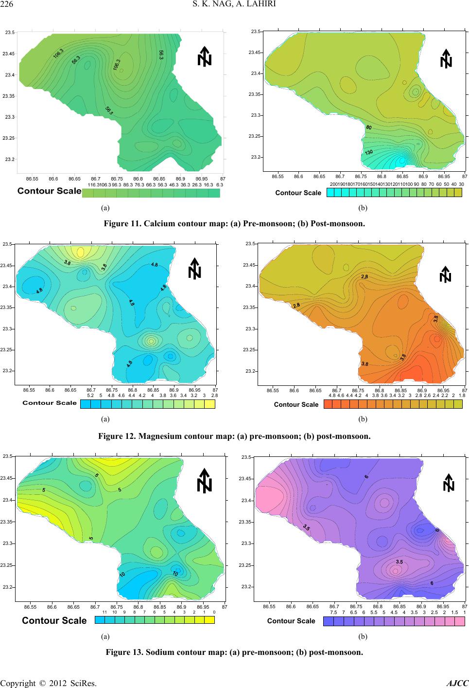 S. K. NAG, A. LAHIRI 226 86.55 86.6 86.65 86.7 86.75 86.8 86.85 86.9 86.9587 23.2 23.25 23.3 23.35 23.4 23.45 23.5 30405060708090100110120130140150160170180190200 Contour Scale (a) (b) Figure 11. Calcium contour map: (a) Pre-monsoon; (b) Post-monsoon. 86.55 86.6 86.65 86.786.75 86.8 86.8586.9 86.9587 23.2 23.25 23.3 23.35 23.4 23.45 23.5 2.833.23.43.63.844.24.44.64.855.2 Contour Scale 86.5586.686.6586.7 86.7586.886.8586.9 86.9587 23.2 23.25 23.3 23.35 23.4 23.5 23.45 1.822.22.42.62.833.23.43.63.844.24.44.64.8 Contour Scale (a) (b) Figure 12. Magnesium contour map: (a) pre-monsoon; (b) post-monsoon. 86.55 86.686.65 86.7 86.75 86.8 86.85 86.9 86.9587 23.2 23.25 23.3 23.35 23.4 23.45 23.5 01234567891011 Contour Scale 86.55 86.686.6586.7 86.75 86.8 86.85 86.9 86.9587 23.2 23.25 23.3 23.35 23.4 23.45 23.5 11.522.533.544.555.566.577.5 Contour Scale (a) (b) Figure 13. Sodium contour map: (a) pre-monsoon; (b) post-monsoon. Copyright © 2012 SciRes. AJCC  S. K. NAG, A. LAHIRI 227 86.55 86.686.65 86.7 86.7586.8 86.85 86.986.9587 23.2 23.25 23.3 23.35 23.4 23.45 23.5 00.20.40.60.811.21.41.61.822.22.42.62.83 Contour Scale 86.55 86.6 86.65 86.786.7586.886.85 86.9 86.9587 23.2 23.25 23.3 23.35 23.4 23.45 23.5 -0.200.20.40.60.811.21.41.61.822.22.42.62.8 Contour Scale (a) (b) Figure 14. Iron contour map: (a) pre-monsoon; (b) post-monsoon. Figure 15. US salinity diagram. Figure 17. Permeability index diagram. 5. Conclus ne of the most important use of groundwater is for drinking purpose. Hence, it is essential to ascertain the quality of groundwater because the presence of some minerals beyond certain limits may be unsuitable for drinking. BIS, Government of India [42] has evolved a set of specifications for water to be used for drinking purposes. These are presented in Table 3 and, when compared with the analyzed samples of the study area, it is found that the groundwater is within the safe category, except for few places where higher values of iron and total hardness exist. In general, it may be stated that groundwater of the study area falls within safe category. Hence, the study has helped to improve understanding of physicochemical parameters of the area for effective management and proper utilizatces for better living conditiononitoring ions O ion of groundwater resour s of the people. A continuous m Figure 16. Wilcox diagram. Copyright © 2012 SciRes. AJCC  S. K. NAG, A. LAHIRI 228 Figure 18. Piper trilinear diagram. Table 3. Comparison of chemical analyses data with BIS, Govt. of India (pre-monsoon and post-monsoon, 2009). Analysed Samples Remarks Sample No. Constituents Limits of General Acceptability Allowable Limit Pre-Monsoon Post-MonsoonPre-Monsoon Post-Monsoon 1. pH 7 - 8 0.5 - 9.2 6 - 8 6.2 - 8.1 Within the limit Within the limit 2. Total Dissolved Solid (mg/L) 500 1500 83 - 1242 92 - 1365 Within the limit Within the limit 3. Specific Conductivity (at 25˚C) µS/cm Below 780 - 140 - 1940 200 - 3400 Satyatan Primary School, Teghari, Gara, and Goaldanga having more than 800 µS/cm. Within the limit 4. Total Hardness (as CaCO3) (mg/L) 300 600 90 - 1190 20 - 1070 Teghari and Gara having more than 1000 mg/L of CaCO3. Satyatan Primary School has 870 mg/L of CaCO3. Teghari and Gara, Dwarkeswar River Bed having more than 1000 mg/L of CaCO3. 5. Calcium (mg/L) 75 200 6.39 - 113.7430.06 - 214.23Within the limit Within the limit 6. Magnessium (mg/L) 50 4.88Within the limit Within the limit Iron (mg/L) 1 Jhatipahari has 3 mg/L of Fe an Kng/L Kamalpur, , nd mankiari has 3 go /L e of Cl in water 150 2.84 - 5.22 1.93 - 7. 0.3 1.0 0. - 30 - 3 Kamalpur, Sukhnibash, Sukhnibash Jhatipahari a d also Da audi, has 1.2 m of Fe in water m/L of Fe and als Kanudi, has 1.2 mg of Fe in water 8. Chloride (mg/L) 200 600 10 - 660 20 - 580 Tghari and Gara has more than 600 mg/LWithin the limit Copyright © 2012 SciRes. AJCC 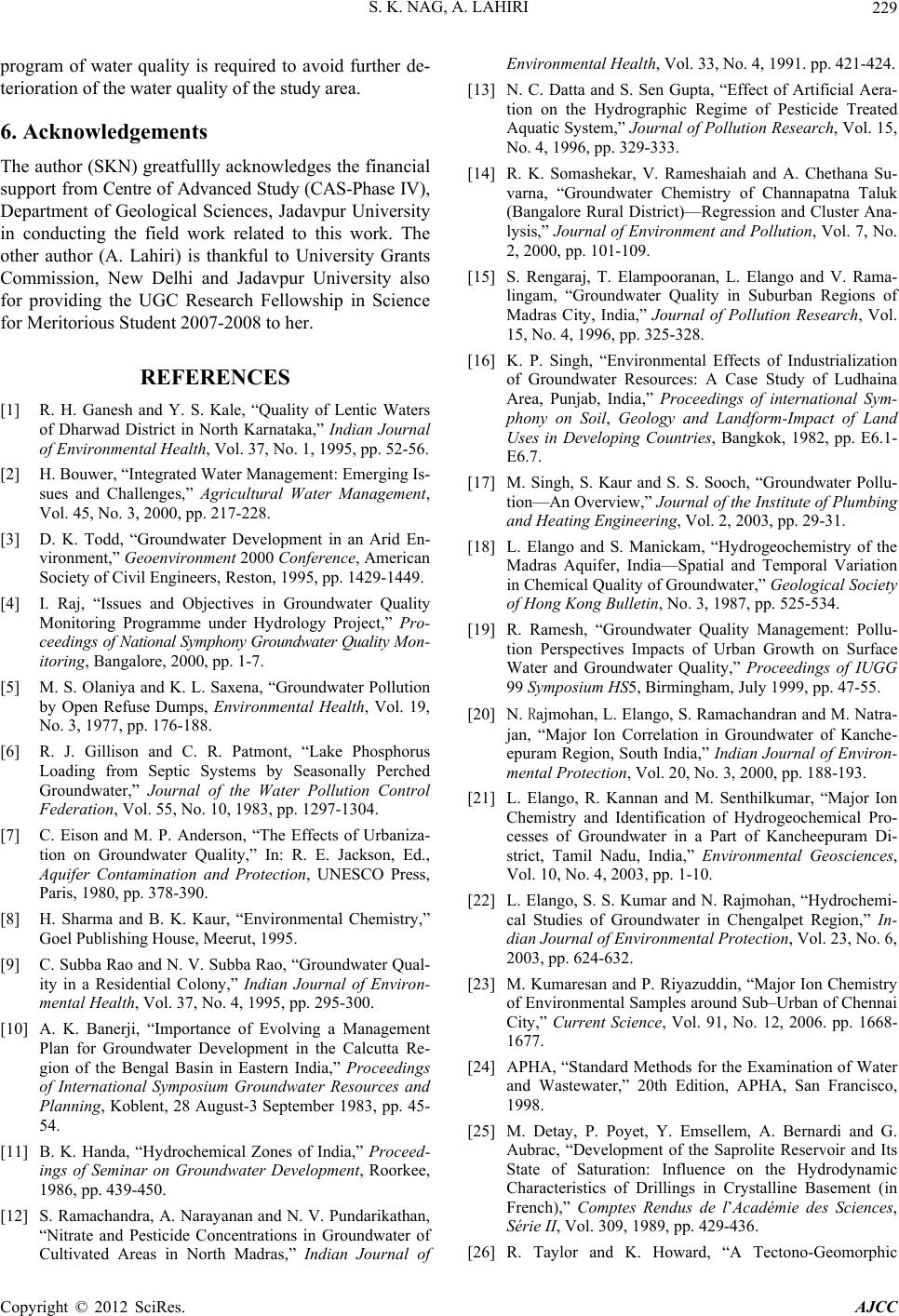 S. K. NAG, A. LAHIRI 229 program of water quality is required to avoid further de- terioratity of the study area. 6. Acknowledgements The author (SKN) greatfullly acknowledges the financial support from Centre of Advanced Study (CAS-Phase IV), Departm Sciencdavpur Ursity in conductinrk related to this work. The other author (A. Lahiri) is thankful to University Grants Cmissi and Jaaur Univso f rovsearch Fellowship in Scienc for Meritorious Student 2007-2008 to her. ERENCES [1] R. H. Ganesh and Y. S. Kale, “Quality of Lentic Waters of Dharwad District in North Karnataka,” Indian Journal of Environmental Health, Vol. 37, No. 1, 1995, pp. 52-56. H. Bouwer, “Integrated Water Mement: Eg Is- sues and Challenges,” Agricultural Water Management, Arid En- vironment,” Geoenvironment 2000 Conference, American Reston, 1995, pp. 1429-1449. onally Perched Groundwater,” Journal of the Water Pollution Control Federation, Vol. 55, No. 104. [7] C. Eison and ffects of Urbaniza- eptember 1983, pp. 45- Environmental Heal, 1991. pp. 421-424. N. C. Datta S. St ion dro Aquatic System,” Jouon Research, Vol. 15, No. 4, 1996, pp. 329-3 [14] R. K. Somashekar, nd- varna, “Groundwa (Baal lysis,” Journal of 2, 2000, pp. 101-10 Rlla- a dialu ool. 15, No. 4, 1996, pp. 32 [16] K. P. Singh, “Envirots ofn of Groundwater RSa Area, Punjab, Ind phony on Soil, G Uses in Developing Countrieso.1- E6.7 [17] M. Singh, S. Kaur mbing . 3, 1987, pp. 525-534. rowth on Surface Natra- s of Groundwater in a Part of Kancheepuram Di- ar and N. Rajmohan, “Hydrochemi- for the Examination of Water Influence on the Hydrodynamic “A Tectono-Geomorphic ion of the water qual ent of Geological g the field wo es, Janive omon, New Delhidvpersity al [15] S. lingam, “Groun or piding the UGC Ree M REF [2] anagmergin Vol. 45, No. 3, 2000, pp. 217-228. [3] D. K. Todd, “Groundwater Development in an [18 Society of Civil Engineers, [4] I. Raj, “Issues and Objectives in Groundwater Quality Monitoring Programme under Hydrology Project,” Pro- ceedings of National Symphony Groundwater Quality Mo n- itoring, Bangalore, 2000, pp. 1-7. [5] M. S. Olaniya and K. L. Saxena, “Groundwater Pollution by Open Refuse Dumps, Environmental Health, Vol. 19, No. 3, 1977, pp. 176-188. [6] R. J. Gillison and C. R. Patmont, “Lake Phosphorus Loading from Septic Systems by Seas jan, , 1983, pp. 1297-130 M. P. Anderson, “The E tion on Groundwater Quality,” In: R. E. Jackson, Ed., Aquifer Contamination and Protection, UNESCO Press, Paris, 1980, pp. 378-390. [8] H. Sharma and B. K. Kaur, “Environmental Chemistry,” Goel Publishing House, Meerut, 1995. [9] C. Subba Rao and N. V. Subba Rao, “Groundwater Qual- cal S ity in a Residential Colony,” Indian Journal of Environ- mental Health, Vol. 37, No. 4, 1995, pp. 295-300. [10] A. K. Banerji, “Importance of Evolving a Management Plan for Groundwater Development in the Calcutta Re- gion of the Bengal Basin in Eastern India,” Proceedings of International Symposium Groundwater Resources and Planning, Koblent, 28 August-3 S and W 54. [11] B. K. Handa, “Hydrochemical Zones of India,” Proceed- ings of Seminar on Groundwater Development, Roorkee, 1986, pp. 439-450. [12] S. Ramachandra, A. Narayanan and N. V. Pundarikathan, “Nitrate and Pesticide Concentrations in Groundwater of Cultivated Areas in North Madras,” Indian Journal of tion—An Overview,” Journal of the Institute of Plu and Heating Engineering, Vol. 2, 2003, pp. 29-31. th, Vol. 33, No. 4 en Gupta, “Effec graphic Regime o rnal of Polluti 33. [13] t and on the Hy of Artificial Aera- f Pesticide Treated V. Rameshaiah a ter Chemistry of C District)—Regressio Environment and Po 9. A. Chethana Su hannapatna Taluk n and Cluster Ana- llution, Vol. 7, No. ngalore Rur engaraj, T. E dwater Qu ampooranan, L. Eango and V. Ram ality in Suburban R ,” Journal of Polegions of tin Research, Vdras City, In 5-328. nmental Effec esources: A Case ia,” Proceedings of eology and Landfo Industrializatio tudy of Ludhain international Sym- rm-Impact of Land k, 1982, pp. E6, Bangk and S. S. Sooch, “Groundwater Pollu- . ] L. Elango and S. Manickam, “Hydrogeochemistry of the Madras Aquifer, India—Spatial and Temporal Variation in Chemical Quality of Groundwater,” Geological Society of Hong Kong Bulletin, No [19] R. Ramesh, “Groundwater Quality Management: Pollu- tion Perspectives Impacts of Urban G Water and Groundwater Quality,” Proceedings of IUGG 99 Symposium HS5, Birmingham, July 1999, pp. 47-55. [20] N. Rajmohan, L. Elango, S. Ramachandran and M. “Major Ion Correlation in Groundwater of Kanche- epuram Region, South India,” Indian Journal of Environ- mental Protection, Vol. 20, No. 3, 2000, pp. 188-193. [21] L. Elango, R. Kannan and M. Senthilkumar, “Major Ion Chemistry and Identification of Hydrogeochemical Pro- cesse strict, Tamil Nadu, India,” Environmental Geosciences, Vol. 10, No. 4, 2003, pp. 1-10. [22] L. Elango, S. S. Kum tudies of Groundwater in Chengalpet Region,” In- dian Journal of Environmental Protection, Vol. 23, No. 6, 2003, pp. 624-632. [23] M. Kumaresan and P. Riyazuddin, “Major Ion Chemistry of Environmental Samples around Sub–Urban of Chennai City,” Current Science, Vol. 91, No. 12, 2006. pp. 1668- 1677. [24] APHA, “Standard Methods astewater,” 20th Edition, APHA, San Francisco, 1998. [25] M. Detay, P. Poyet, Y. Emsellem, A. Bernardi and G. Aubrac, “Development of the Saprolite Reservoir and Its State of Saturation: Characteristics of Drillings in Crystalline Basement (in French),” Comptes Rendus de l’Académie des Sciences, Série II, Vol. 309, 1989, pp. 429-436. [26] R. Taylor and K. Howard, Copyright © 2012 SciRes. AJCC 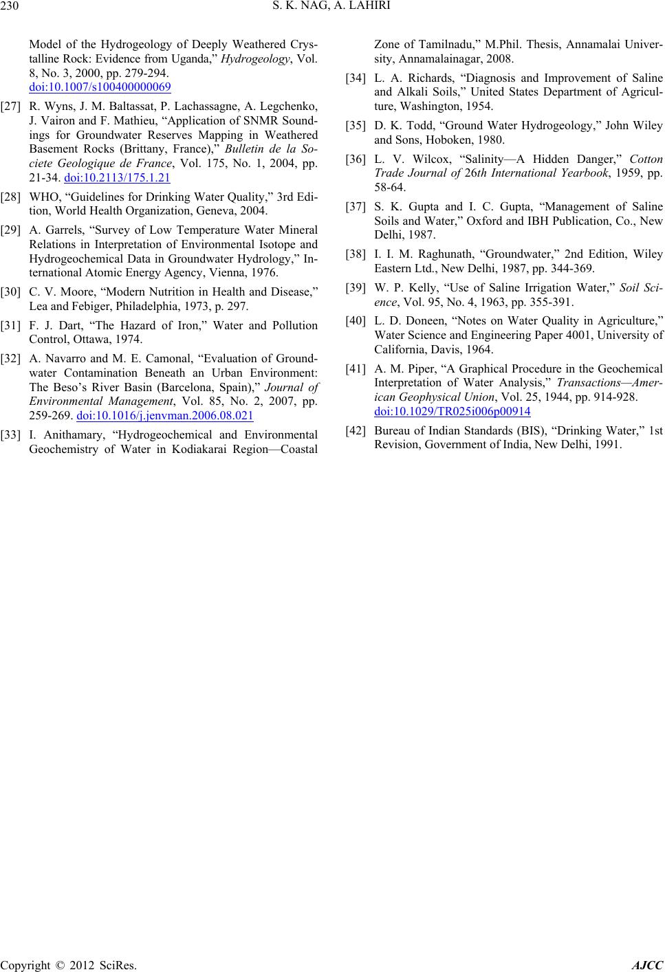 S. K. NAG, A. LAHIRI 230 Model of the Hydrogeology of Deeply Weathered Crys- talline Rock: Evidence from Uganda,” Hydrogeology, Vol. 8, No. 3, 2000, pp. 279-294. doi:10.1007/s100400000069 [27] R. Wyns, J. M. Baltassat, P. Lachassagne, A. Legchenko, J. Vairon and F. Mathieu, “Application of SNMR Sound- 4, pp ings for Groundwater Reserves Mapping in Weathered Basement Rocks (Brittany, France),” Bulletin de la So- ciete Geologique de France, Vol. 175, No. 1, 200. 21-34. doi:10.2113/175.1.21 [28] WHO, “Guidelines for Drinking Water Quality,” 3rd Edi- tion, World Health Organization, Geneva, 2004. [29] A. Garrels, “Survey of Low Temperature Water Mineral Relations in Interpretation of Environmental Isotope and Hydrogeochemical Data in Groundwater Hydrology,” In- ternational Atomic Energy Agency, Vienna, 1976. [30] C. V. Moore, “Modern Nutrition in Health and Disease,” Lea and Febiger, Philadelphia, 1973, p. 297. [31] F. J. Dart, “The Hazard of Iron,” Water and Pollution Control, Ottawa, 1974. [32] A. Navarro and M. E. Camonal, “Evaluation of Ground- water Contamination Beneath an Urban Environment: The Beso’s River Basin (Barcelona, Spain),” Journal of Environmental Management, Vol. 85, No. 2, 2007, pp. 259-269. doi:10.1016/j.jenvman.2006.08.021 [33] I. Anithamary, “Hydrogeochemical and Environmental Geochemistry of Water in Kodiakarai Region—Coastal Zone of Tamilnadu,” M.Phil. Thesis, Annamalai Univer- sity, Annamalainagar, 2008. [34] L. A. Richards, “Diagnosis and Improvement of Saline and Alkali Soils,” United States Department of Agricul- n Wiley n, Co., New roundwater,” 2nd Edition, Wiley ture, Washington, 1954. [35] D. K. Todd, “Ground Water Hydrogeology,” Joh and Sons, Hoboken, 1980. [36] L. V. Wilcox, “Salinity—A Hidden Danger,” Cotton Trade Journal of 26th International Yearbook, 1959, pp. 58-64. [37] S. K. Gupta and I. C. Gupta, “Management of Saline Soils and Water,” Oxford and IBH Publicatio Delhi, 1987. [38] I. I. M. Raghunath, “G Eastern Ltd., New Delhi, 1987, pp. 344-369. [39] W. P. Kelly, “Use of Saline Irrigation Water,” Soil Sci- ence, Vol. 95, No. 4, 1963, pp. 355-391. [40] L. D. Doneen, “Notes on Water Quality in Agriculture,” Water Science and Engineering Paper 4001, University of California, Davis, 1964. [41] A. M. Piper, “A Graphical Procedure in the Geochemical Interpretation of Water Analysis,” Transactions—Amer- ican Geophysical Union, Vol. 25, 1944, pp. 914-928. doi:10.1029/TR025i006p00914 [42] Bureau of Indian Standards (BIS), “Drinking Water,” 1st Revision, Government of India, New Delhi, 1991. Copyright © 2012 SciRes. AJCC |