American Journal of Climate Change, 2012, 1, 194-204
http://dx.doi.org/10.4236/ajcc.2012.14016 Published Online December 2012 (http://www.SciRP.org/journal/ajcc)
Measuring Capacity for Resilience among Coastal
Counties of the US Northern Gulf of Mexico Region
Margaret A. Reams, Nina S. N. Lam, Ariele Baker
Department of Environmental Sciences, Louisiana State University, Baton Rouge, USA
Received September 27, 2012; revised October 27, 2012; accepted November 9, 2012
ABSTRACT
Many have voiced concern about the long-term survival of coastal communities in the face of increasingly intense
storms and sea level rise. In this study we select indicators of key theoretical concepts from the social-ecological resi-
lience literature, aggregate those indicators into a resilience-capacity index, and calculate an index score for each of the
52 coastal counties of Louisiana, Texas, Mississippi, Alabama and Florida. Building upon Cutter’s Social Vulnerability
Index work [1], we use Factor Analysis to combine 43 variables measuring demographics, social capital, economic re-
sources, local government actions, and environmental conditions within the counties. Then, we map the counties’ scores
to show the spatial distribution of resilience capacities. The counties identified as having the highest resilience capaci-
ties include the suburban areas near New Orleans, Louisiana and Tampa, Florida, and the growing beach-tourist com-
munities of Alabama and central Florida. Also, we examine whether those counties more active in oil and gas develop-
ment and production, part of the region’s “energy coast”, have greater capacity for resilience than other counties in the
region. Correlation analyses between the resilience-capacity index scores and two measures of oil and gas industry ac-
tivity (total employment and number of business establishments within five industry categories) yielded no statistically
significant associations. By aggregating a range of important contextual variables into a single index, the study demon-
strates a useful approach for the more systematic examination and comparison of exposure, vulnerability and capacity
for resilience among coastal communities.
Keywords: Community Resilience; Vulnerability; Sea Level Rise; Coastal Hazards; Hurricanes; Oil and Gas Industry
1. Introduction
In the years since Hurricanes Katrina and Rita in 2005,
scholars, policy makers, residents and other stakeholders
have raised questions about the long-term survival of
coastal communities in the face of increasingly intense
storms, sea-level rise and other natural hazards. The
residents in the study area, the coastal communities of
the Northern Gulf of Mexico Region, live with threats to
their safety and to the longer-term social and economic
stability of their communities. Coastal hazards include
both large-scale, rapid-moving disruptive events such as
hurricanes and storm surges, and slower-moving distur-
bances, such as coastal land loss, sea-level rise, and the
gradual diminishment of ecosystem services over time.
While many coastal threats result from or are associ-
ated with natural processes, most are exacerbated by hu-
man activities, such as rapid population growth, inade-
quate infrastructure planning and investment, and unwise
land-use decisions. Theorists and community stakehold-
ers would benefit from a resilience assessment instru-
ment that would provide them with information about
their vulnerabilities, and their capacity for taking adap-
tive steps to make their communities safer and more
likely to recover following large-scale disturbances.
Despite abundant research examining aspects of so-
cial-ecological resilience, vulnerability, hazards and risk
assessment, there is not yet a convincing approach to
quantifying and measuring community resilience. Our
research objectives are to develop quantitative indicators
of capacity for resilience to coastal hazards, compile
these indicators into an index, and make comparisons
among the counties. We are particularly interested in
whether the coastal counties considered to be part of the
Gulf of Mexico’s “energy coast”—those most directly
involved with off-shore and on-shore oil and gas energy
development and production—may have greater resi-
lience capacities than other coastal counties in the region.
The challenges involved in developing useful resi-
lience indices are significant [2-5]. Some appear to arise,
in part, due to the various definitions of resilience used
by researchers. The definitions are often confused or
used interchangeably with similar concepts such as vul-
nerability, sustainability, and adaptability. Also the pro-
blem is exacerbated by a lack of empirical validation and
C
opyright © 2012 SciRes. AJCC

M. A. REAMS ET AL. 195
evidence for the indices derived [6]. Moreover, most of
the literature on resilience tends to be conceptual and
somewhat abstract. A straight-forward model for meas-
uring resilience capacity that is grounded in sound theo-
retical principles will be very useful for sustainable plan-
ning and management and may help speed economic
assistance and recovery of communities after major di-
saster events.
The theoretical foundation for this study comes from
the growing body of scholarly research concerning so-
cial-ecological resilience, hazard and vulnerability, and
coupled natural and human systems [1,7,8]. In summa-
rizing the related research in the literature below, our
discussion focuses on two issues: what is community
resilience and how can it best be measured?
2. Related Research
2.1. Definition of Social Ecological Resilience
Some researchers define resilience as how fast a system
can return to the original state after an external distur-
bance, while others use the term to refer to how far the
system could be perturbed without shifting to a different
state. The former definition often is called engineering
resilience as it concerns with the return time, whereas the
latter is commonly referred to as ecological resilience [9]
[3]. Adger and colleagues [7] further elaborated that:
“Resilience reflects the degree to which a complex adap-
tive system is capable of self-organization (emphasis
added), and the degree to which the system can build
capacity for learning and adaptation (emphasis added).”
They further defined resilience as “the capacity of linked
social-ecological systems to absorb recurrent distur-
bances such as hurricanes or floods so as to retain essen-
tial structures, processes, and feedbacks”.
Based on the literature, we can summarize that the best
working definition of resilience would include three
characteristics: 1) the magnitude of shock a system can
absorb and remain within a given state; 2) the degree to
which the system is capable of self organization, and 3)
the degree to which the given system can build capacity
for learning and adaptation [10-12].
Closely related to resilience is the concept of vulner-
ability. In fact, the two terms have been used inter-
changeably by some researchers, while others expanded
the definition of vulnerability to include resilience. For
example, Folke and colleagues [10] defined vulnerability
in an ecological sense as “the propensity of an ecological
system to suffer harm from exposure to external stresses
and shocks”, while Cutter and colleagues’ [1] definition
focused on vulnerability within a social system. They de-
fined social vulnerability as “a measure of both the sensi-
tivity of a population to natural hazards and its ability to
respond and recover from the impacts of hazards”. Adger
[13] considered vulnerability in a system to include both
social and ecological elements, and referred to it as the
susceptibility to risk and its inability to cope with or ab-
sorb a shock. Turner and others [14] stressed that vul-
nerability is not just exposure to hazards; it includes three
elements: exposure, sensitivity, and resilience. They fur-
ther suggested that their expanded framework of vulner-
ability and vulnerability analysis can be used for the as-
sessment of coupled human and natural systems and is a
key element of “sustainability science” [8,14]. A similar
conceptual framework is found in the work of [15]
Kasperson and colleagues [15], and Cutter and others [1],
as well.
Various factors may increase social vulnerability, in-
cluding exclusion of stakeholders from the public policy
arena, an incorrect understanding of ecosystem processes
and risks associated with natural hazard, and inadequate
plans for disaster management and response. Further,
lower income residents may tend to live in riskier areas
in urban settlements making them more vulnerable to
flooding, disease and chronic stresses. Also, women have
been found to be at increased risks associated with envi-
ronmental hazards, often including a disproportionate
share of the work related to the recovery of home and
livelihood after an event [13,16]. Thus, potential influ-
ences on social vulnerability include age, gender, race
and socioeconomic status, special needs population or
those that lack normal social safety nets during disaster
recovery, and the quality and density of the built envi-
ronment [1].
2.2. Measuring Community Resilience
While there is voluminous literature on the conceptual
frameworks, definitions, and case studies related to com-
munity resilience, few attempts have been made to quan-
tify resilience and/or vulnerability. There are major chal-
lenges associated with quantifying resilience. First, the
numerous definitions of the terms, as discussed above,
reflect how different researchers may consider and select
indicators differently for measuring resilience. Thus, the
selection of appropriate indicators for measurement be-
comes a major task. Mathematical and statistical methods
will be needed to identify and evaluate the key factors
iteratively, and the resultant measurement model will
need to be tested and verified.
Second, there is a need to consider both social and
natural aspects of resilience, and how these two systems
are linked. A system that has high social resilience may
have low ecological resilience and vice versa. Moreover,
the interaction effects between the two systems may be
exhibited at different points in time, making them diffi-
cult to measure. For example, building a levee along the
Mississippi River would prevent flooding to the populated

M. A. REAMS ET AL.
196
areas, hence decreasing the vulnerability of the people
living in low-lying areas. However, such action may lead
to increased vulnerability of the wetland ecosystem be-
cause of long-term reduction in sediment load, leading to
an increase in wetland erosion. This consequence can in
turn become a threat to the human system, because the
loss of wetlands would reduce the buffer zone that pro-
tects the populated areas and increases the vulnerability
of communities to hurricanes. This type of coupling
mechanism is easy to describe but is hard to quantify,
especially when useful longitudinal data are not avail-
able.
Third, of those who have attempted to measure vul-
nerability and resilience, the results have seldom been
validated. Often times, the model specification and the
weights assigned to different variables were arbitrarily
determined, making the resultant model difficult to apply
and generalize. We present below three studies of meas-
uring vulnerability and resilience, which will further il-
lustrate the difficulties in measuring resilience and/or
vulnerability.
Yusuf and Francisco [17] developed a model to assess
the vulnerability of sub-national areas in Southeast Asia
to climate change. They followed the definition devel-
oped by the United Nations’ Inter-governmental Panel on
Climate Change [18], which defined vulnerability (V) as
a function of exposure (E), sensitivity (S), and adaptive
capacity (C):


,, .VfESC (1)
Exposure refers to the nature and degree to which a
system is exposed to significant climatic variations, sen-
sitivity means the degree to which a system is affected by
climate-related events, and adaptive capacity is the abili-
ty of a system to adjust to climate change or to cope with
its consequences. Their model is an additive weighted-
average model. The weight of each variable was assigned
arbitrarily according to the literature. The results from
their study are the composite vulnerability index of each
sub-national region in the Southeast Asia. While their ap-
proach is straight-forward and the resultant maps are im-
pressive, the study suffers from the pitfalls discussed
above, namely the lack of empirical verification of model
results and the arbitrariness of weight assignments.
A similar but improved approach to the above IPCC
vulnerability model was used recently to measure the
vulnerability of Australian rural communities to climate
variability and change [19,20]. The research group recog-
nized that the concept of vulnerability is rarely converted
to quantitative measures that can be used to prioritize
policy interventions and evaluate their impacts. In de-
veloping their vulnerability index, the researchers em-
phasized the need to include some measures of adaptive
capacity to complement the existing hazard-impact mo-
deling. An adaptive-capacity index was created using the
rural livelihood analysis framework proposed by Ellis
[21] that includes indicators from the five categories of
resources or “capitals”: human, social, natural, physical,
and financial.
The third example is the approach used and pioneered
by Cutter and her research group to quantify the social
aspects of vulnerability into the Social Vulnerability In-
dex [1,22,23]. The group has used the index to evaluate
the social vulnerability of the entire United States, the
coastal counties of the United States, and the relative
impacts of Hurricane Katrina on the Gulf Coast. To de-
velop the index, Cutter and others selected 42 socioeco-
nomic variables from the US Census that demonstrated
aspects of social vulnerability as identified by the litera-
ture. They conducted a factor analysis in the form of
principal component analysis to derive 11 factors that
accounted for 76.4% of variance of all the variables. The
relative index of vulnerability for each county was de-
rived by adding their factor scores, and the final index
was mapped using standard deviations from the mean
score to determine level of vulnerability. Those counties
with the highest standard deviations from the mean were
described as the most vulnerable while those with the
lowest standard deviations were described as the least
vulnerable.
In order to verify the accuracy of the index, Cutter and
the group correlated the number of presidential disaster
declarations with the vulnerability score given to each
county. The result was disappointing; they found literally
no correlation (r = −0.099) between the derived vulner-
ability index and the political designations. Nevertheless,
Cutter’s approach has advanced two important concepts
regarding the measurement of resilience or vulnerability,
which are, the need to derive the index through statistical
modeling and the need to validate the index through em-
pirical comparisons with outcomes such as the number of
disaster declarations.
3. Resilience-Capacity Index Calculation
3.1. Study Area and Data
The focus of this study is the northern Gulf of Mexico
region, specifically the coastal counties of Texas, Louisiana,
Mississippi, Alabama and Florida. Counties selected for
this study have some part of their land mass bordering
the Gulf of Mexico. A total of 52 counties met this selec-
tion criterion and were used in this analysis.
Demographic and economic data used in this study
were gathered from the US Census Bureau 2000 Census
of Population, and the 1997 and 2002 Economic Census.
The data were obtained from the website
http://factfin- der.census.gov/home/saff/main.html?_lang
=en.Environ-mental data were obtained in two different

M. A. REAMS ET AL. 197
ways that will be discussed in more detail in the next
section. Toxic Release Inventory (TRI) data from 2000
were obtained from the US Environmental Protection
Agency from the website: http://iaspub.epa.gov/triexplor-
er/tri_release.facility. Digital elevation measures were
available through the USGS seamless map server at the
website http://seamless.usgs.gov.
3.2. The Factor Analysis Method
As introduced above, the social aspects of vulnerability
were first quantified by Cutter and colleagues [1]. They
developed the Social Vulnerability Index by selecting 42
socioeconomic indicators of social vulnerability and con-
ducting a factor analysis in the form of principal compo-
nent analysis (PCA) to create an index of these variables
to measure social vulnerability.
There are a few ways in which Cutter’s method could
be improved. First the factor analysis method might be
changed. Instead of using a principal component analysis
to create the factors a principal axis factoring method
could be used. A principal component analysis seeks to
explain all the common and unique variance of the vari-
ables, while a principal axis factoring method seeks only
to explain the common variances. Secondly, a principal
component analysis is a variance-based approach while
principal axis factoring is a correlation-focused approach.
This means that in a principal axis factoring method
every variable is included in the analysis, yet not every
variable is deemed important. In other words, a principal-
axis factoring method acts as a filter while a principal
component analysis includes all the variables [24].
Secondly, factor scores are the sum of positive and
negative values of variables around an axis for a case.
They are in themselves an index of the relationship of
indicators to each other. Therefore, to create an index of
factor scores is to include all variables into the index, and
create an index of an index. This can be impractical and
hard to manage. As an alternative, could the factor ana-
lysis provide a methodology to discern which variables
aremost important to each dimension or factor instead of
using factor scores?
Thirdly, Cutter et al. [1] made no a priori assumptions
about importance. They used an additive model that did
not weight the variance explained by each factor. Each
factor explains a percent of the variance (i.e. eigenvalue)
within the data matrix and this varies based on the rela-
tionship of the variables to each other within each factor.
Therefore each factor should be weighted to its relative
importance, and this is statistically determined when the
factors are calculated.
3.3 A Modified Method to Create the Resilience
Index
The methods used by Cutter et al. [1] to create the Social
Vulnerability Index were modified to create an index of
community capacity for resilience. Socioeconomic vari-
ables were obtained from the 2000 Census, 36 of these
variables were taken from the research of Cutter and col-
leagues and 7 new variables were added that measured
additional aspects of vulnerability and resilience, includ-
ing voting rates among residents, economic resources of
local government, and environmental factors. All vari-
ables used in this analysis are shown in Table 1.
The variables taken from Cutter et al. [1] were se-
lected because they measure generally accepted aspects
of social vulnerability. These concepts include: limited
access to economic resources and political power, fewer
social networks, less structurally sound housing, and
more physically limited individuals. Specific variables
that identify these measures of vulnerability are age,
gender, race and socioeconomic status. Other measures
of the social capital of a community include housing type
and abundance, rental properties and housing values.
Measures of the economic conditions of the area include
commercial development, manufacturing density, earn-
ing density, and primary employments in an area. Sup-
plemental Security Income (SSI) recipients were added
as an additional measure of economic vulnerability.
We added variables concerning voting rates among
residents and local government spending, as well, be-
cause these factors may affect a community’s ability to
adapt and/or mitigate the damages associated with coa-
stal disturbances. Additional variables that measure en-
vironmental attributes and conditions were added be-
cause they relate to the residents’ exposure to hazards.
These variables included Toxic Release Inventory (TRI)
values and the mean elevation of the county. The TRI
reflects the estimated discharges of TRI-listed chemicals
within each county and were included because they offer
insight into local environmental conditions. Elevation
was used because it indicates susceptibility to flooding, a
relevant consideration in coastal, hurricane-prone areas.
The Toxic Release Inventory (TRI) data was obtained
from the EPA website using the TRI Explorer tool. Re-
lease reports were selected for 2000. The data was se-
lected by county, and total on site or offsite disposal or
other releases with chemical name was used to obtain a
measure of toxic pollution per county for all chemicals
across all industries. These numbers were listed in of
pounds. Data in the year 2000 ranged from: 0 releases of
any chemical in Kleberg, TX, to 55,247,688 lbs in Es-
cambia County, Florida. The median value of TRI re-
lease in the Gulf of Mexico region in the year 2000 was
283,910 lbs of Toxic releases.
The variable “mean elevation” was obtained through a
multistep process. First, data was downloaded from the
USGS Seamless Map Server Program in a Digital Eleva-
tion Model format (DEM) for all the coastal counties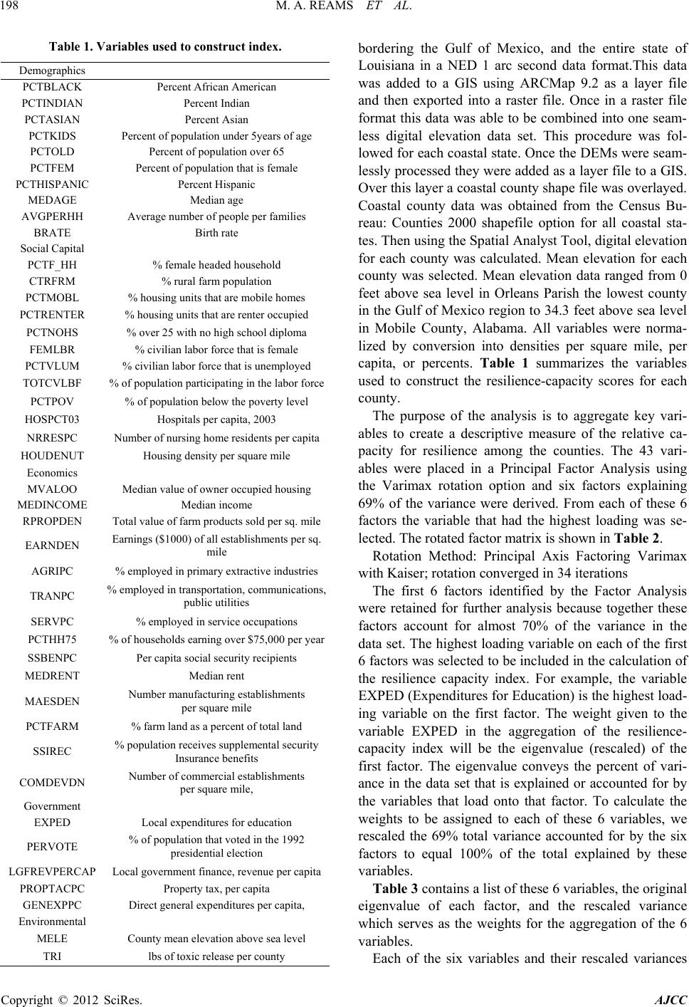

M. A. REAMS ET AL.
198
Table 1. Variables used to construct index.
Demographics
PCTBLACK Percent African American
PCTINDIAN Percent Indian
PCTASIAN Percent Asian
PCTKIDS Percent of population under 5years of age
PCTOLD Percent of population over 65
PCTFEM Percent of population that is female
PCTHISPANIC Percent Hispanic
MEDAGE Median age
AVGPERHH Average number of people per families
BRATE Birth rate
Social Capital
PCTF_HH % female headed household
CTRFRM % rural farm population
PCTMOBL % housing units that are mobile homes
PCTRENTER % housing units that are renter occupied
PCTNOHS % over 25 with no high school diploma
FEMLBR % civilian labor force that is female
PCTVLUM % civilian labor force that is unemployed
TOTCVLBF % of population participating in the labor force
PCTPOV % of population below the poverty level
HOSPCT03 Hospitals per capita, 2003
NRRESPC Number of nursing home residents per capita
HOUDENUT Housing density per square mile
Economics
MVALOO Median value of owner occupied housing
MEDINCOME Median income
RPROPDEN Total value of farm products sold per sq. mile
EARNDEN Earnings ($1000) of all establishments per sq.
mile
AGRIPC % employed in primary extractive industries
TRANPC % employed in transportation, communications,
public utilities
SERVPC % employed in service occupations
PCTHH75 % of households earning over $75,000 per year
SSBENPC Per capita social security recipients
MEDRENT Median rent
MAESDEN Number manufacturing establishments
per square mile
PCTFARM % farm land as a percent of total land
SSIREC % population receives supplemental security
Insurance benefits
COMDEVDN Number of commercial establishments
per square mile,
Government
EXPED Local expenditures for education
PERVOTE % of population that voted in the 1992
presidential election
LGFREVPERCAP Local government finance, revenue per capita
PROPTACPC Property tax, per capita
GENEXPPC Direct general expenditures per capita,
Environmental
MELE County mean elevation above sea level
TRI lbs of toxic release per county
bordering the Gulf of Mexico, and the entire state of
Louisiana in a NED 1 arc second data format.This data
was added to a GIS using ARCMap 9.2 as a layer file
and then exported into a raster file. Once in a raster file
format this data was able to be combined into one seam-
less digital elevation data set. This procedure was fol-
lowed for each coastal state. Once the DEMs were seam-
lessly processed they were added as a layer file to a GIS.
Over this layer a coastal county shape file was overlayed.
Coastal county data was obtained from the Census Bu-
reau: Counties 2000 shapefile option for all coastal sta-
tes. Then using the Spatial Analyst Tool, digital elevation
for each county was calculated. Mean elevation for each
county was selected. Mean elevation data ranged from 0
feet above sea level in Orleans Parish the lowest county
in the Gulf of Mexico region to 34.3 feet above sea level
in Mobile County, Alabama. All variables were norma-
lized by conversion into densities per square mile, per
capita, or percents. Table 1 summarizes the variables
used to construct the resilience-capacity scores for each
county.
The purpose of the analysis is to aggregate key vari-
ables to create a descriptive measure of the relative ca-
pacity for resilience among the counties. The 43 vari-
ables were placed in a Principal Factor Analysis using
the Varimax rotation option and six factors explaining
69% of the variance were derived. From each of these 6
factors the variable that had the highest loading was se-
lected. The rotated factor matrix is shown in Table 2.
Rotation Method: Principal Axis Factoring Varimax
with Kaiser; rotation converged in 34 iterations
The first 6 factors identified by the Factor Analysis
were retained for further analysis because together these
factors account for almost 70% of the variance in the
data set. The highest loading variable on each of the first
6 factors was selected to be included in the calculation of
the resilience capacity index. For example, the variable
EXPED (Expenditures for Education) is the highest load-
ing variable on the first factor. The weight given to the
variable EXPED in the aggregation of the resilience-
capacity index will be the eigenvalue (rescaled) of the
first factor. The eigenvalue conveys the percent of vari-
ance in the data set that is explained or accounted for by
the variables that load onto that factor. To calculate the
weights to be assigned to each of these 6 variables, we
rescaled the 69% total variance accounted for by the six
factors to equal 100% of the total explained by these
variables.
Table 3 contains a list of these 6 variables, the original
eigenvalue of each factor, and the rescaled variance
which serves as the weights for the aggregation of the 6
variables.
Each of the six variables and their rescaled variances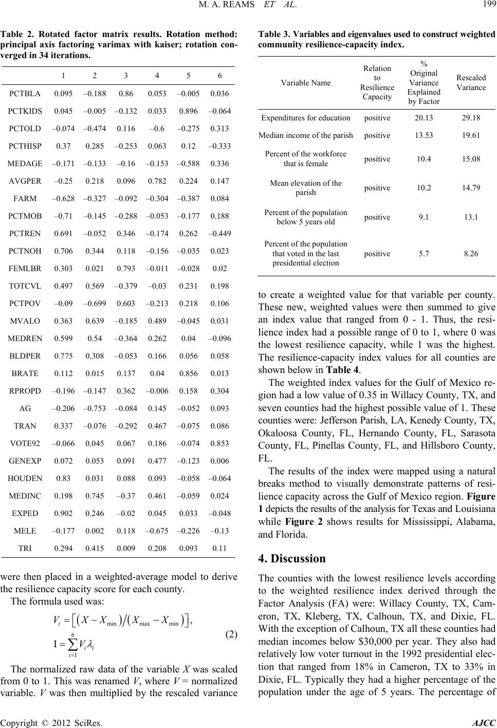

M. A. REAMS ET AL. 199
Table 2. Rotated factor matrix results. Rotation method:
principal axis factoring varimax with kaiser; rotation con-
verged in 34 iterations.
1 2 3 4 5 6
PCTBLA 0.095 ‒0.188 0.86 0.053 ‒0.005 0.036
PCTKIDS 0.045 ‒0.005 ‒0.132 0.033 0.896 ‒0.064
PCTOLD ‒0.074 ‒0.474 0.116 ‒0.6 ‒0.275 0.313
PCTHISP 0.37 0.285 ‒0.253 0.063 0.12 ‒0.333
MEDAGE ‒0.171 ‒0.133 ‒0.16 ‒0.153 ‒0.588 0.336
AVGPER ‒0.25 0.218 0.096 0.782 0.2240.147
FARM ‒0.628 ‒0.327 ‒0.092 ‒0.304 ‒0.387 0.084
PCTMOB ‒0.71 ‒0.145 ‒0.288 ‒0.053 ‒0.177 0.188
PCTREN 0.691 ‒0.052 0.346 ‒0.174 0.262 ‒0.449
PCTNOH 0.706 0.344 0.118 ‒0.156 ‒0.035 0.023
FEMLBR 0.303 0.021 0.793 ‒0.011 ‒0.0280.02
TOTCVL 0.497 0.569 ‒0.379 ‒0.03 0.231 0.198
PCTPOV ‒0.09 ‒0.699 0.603 ‒0.213 0.2180.106
MVALO 0.363 0.639 ‒0.185 0.489 ‒0.045 0.031
MEDREN 0.599 0.54 ‒0.364 0.262 0.04 ‒0.096
BLDPER 0.775 0.308 ‒0.053 0.166 0.0560.058
BRATE 0.112 0.015 0.137 0.04 0.8560.013
RPROPD ‒0.196 ‒0.147 0.362 ‒0.006 0.1580.304
AG ‒0.206 ‒0.753 ‒0.084 0.145 ‒0.052 0.093
TRAN 0.337 ‒0.076 ‒0.292 0.467 ‒0.075 0.086
VOTE92 ‒0.066 0.045 0.067 0.186 ‒0.074 0.853
GENEXP 0.072 0.053 0.091 0.477 ‒0.123 0.006
HOUDEN 0.83 0.031 0.088 0.093 ‒0.058 ‒0.064
MEDINC 0.198 0.745 ‒0.37 0.461 ‒0.059 0.024
EXPED 0.902 0.246 ‒0.02 0.045 0.033‒0.048
MELE ‒0.177 0.002 0.118 ‒0.675 ‒0.226 ‒0.13
TRI 0.294 0.415 0.009 0.208 0.0930.11
were then placed in a weighted-average model to derive
the resilience capacity score for each county.
The formula used was:



minmax min
6
1
,
I
i
ii
i
VXX XX
V 


 




(2)
The normalized raw data of the variable X was scaled
from 0 to 1. This was renamed V, where V = normalized
variable. V was then multiplied by the rescaled variance
Table 3. Variables and eigenvalues used to construct weighted
community resilience-capacity index.
Variable Name
Relation
to
Resilience
Capacity
%
Original
Variance
Explained
by Factor
Rescaled
Variance
Expenditures for educationpositive 20.13 29.18
Median income of the parishpositive 13.53 19.61
Percent of the workforce
that is female positive 10.4 15.08
Mean elevation of the
parish positive 10.2 14.79
Percent of the population
below 5 years old positive 9.1 13.1
Percent of the population
that voted in the last
presidential election
positive 5.7 8.26
to create a weighted value for that variable per county.
These new, weighted values were then summed to give
an index value that ranged from 0 - 1. Thus, the resi-
lience index had a possible range of 0 to 1, where 0 was
the lowest resilience capacity, while 1 was the highest.
The resilience-capacity index values for all counties are
shown below in Table 4.
The weighted index values for the Gulf of Mexico re-
gion had a low value of 0.35 in Willacy County, TX, and
seven counties had the highest possible value of 1. These
counties were: Jefferson Parish, LA, Kenedy County, TX,
Okaloosa County, FL, Hernando County, FL, Sarasota
County, FL, Pinellas County, FL, and Hillsboro County,
FL.
The results of the index were mapped using a natural
breaks method to visually demonstrate patterns of resi-
lience capacity across the Gulf of Mexico region. Figure
1 depicts the results of the analysis for Texas and Louisiana
while Figure 2 shows results for Mississippi, Alabama,
and Florida.
4. Discussion
The counties with the lowest resilience levels according
to the weighted resilience index derived through the
Factor Analysis (FA) were: Willacy County, TX, Cam-
eron, TX, Kleberg, TX, Calhoun, TX, and Dixie, FL.
With the exception of Calhoun, TX all these counties had
median incomes below $30,000 per year. They also had
relatively low voter turnout in the 1992 presidential elec-
tion that ranged from 18% in Cameron, TX to 33% in
Dixie, FL. Typically they had a higher percentage of the
population under the age of 5 years. The percentage of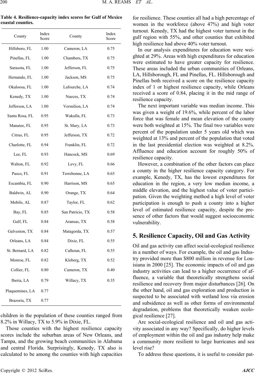

M. A. REAMS ET AL.
200
Table 4. Resilience-capacity index scores for Gulf of Mexico
coastal counties.
County Index
Score County Index Score
Hillsboro, FL 1.00 Cameron, LA 0.75
Pinellas, FL 1.00 Chambers, TX 0.75
Sarasota, FL 1.00 Jefferson, FL 0.75
Hernando, FL 1.00 Jackson, MS 0.75
Okaloosa, FL 1.00 Lafourche, LA 0.74
Kenedy, TX 1.00 Nueces, TX 0.74
Jefferson, LA 1.00 Vermilion, LA 0.74
Santa Rosa, FL 0.95 Wakulla, FL 0.73
Manatee, FL 0.95 St. Mary, LA 0.73
Citrus, FL 0.95 Jefferson, TX 0.72
Charlotte, FL 0.94 Franklin, FL 0.72
Lee, FL 0.93 Hancock, MS 0.69
Walton, FL 0.92 Levy, FL 0.66
Pasco, FL 0.91 Terrebonne, LA 0.65
Escambia, FL 0.90 Harrison, MS 0.65
Baldwin, AL 0.90 Orange, TX 0.64
Mobile, AL 0.87 Taylor, FL 0.62
Bay, FL 0.85 San Patricio, TX 0.58
Gulf, FL 0.84 Aransas, TX 0.58
Galveston, TX 0.84 Matagorda, TX 0.57
Orleans, LA 0.84 Dixie, FL 0.55
St. Bernard, LA 0.82 Calhoun, FL 0.55
Monroe, FL 0.82 Kleberg, TX 0.52
Collier, FL 0.80 Cameron, TX 0.40
Iberia, LA 0.79 Willacy, TX 0.35
Plaquemines, LA 0.77
Brazoria, TX 0.77
children in the population of these counties ranged from
8.2% in Willacy, TX to 5.9% in Dixie, FL.
Those counties with the highest resilience capacity
scores include the suburban areas of New Orleans, and
Tampa, and the growing beach communities in Alabama
and central Florida. Surprisingly, Kenedy, TX also is
calculated to be among the counties with high capacities
for resilience. These counties all had a high percentage of
women in the workforce (above 47%) and high voter
turnout. Kenedy, TX had the highest voter turnout in the
gulf region with 55%, and other counties that exhibited
high resilience had above 40% voter turnout.
In our analysis expenditures for education were wei-
ghted at 29%. Areas with high expenditures for education
were estimated to have greater capacity for resilience.
These areas included the urban communities of Orleans,
LA, Hillsborough, FL and Pinellas, FL. Hillsborough and
Pinellas both received a score on the resilience capacity
index of 1 or highest resilience capacity, while Orleans
received a score of 0.84, placing it in the mid range of
resilience capacity.
The next important variable was median income. This
was given a weight of 19.6%, while percent of the labor
force that was female and mean elevation of the county
were both weighted at 15%. The final two variables were
percent of the population under 5 years old which was
weighted at 13% and percent of the population that voted
in the last presidential election was weighted at 8.2%.
Affluence and education account for roughly 50% of
resilience capacity.
However, a combination of the other factors can place
a county in the higher resilience capacity category. For
example, Kenedy, TX, has the lowest expenditures for
education in the region, a very low median income, a
middle elevation, and the highest value of voter partici-
pation. Given the weighting method a high level of voter
participation is enough to push a county into a higher
level of estimated resilience capacity, despite the pre-
sence of other factors that would suggest socioeconomic
vulnerability.
5. Resilience Capacity, Oil and Gas Activity
Oil and gas activity can affect social-ecological resilience
in a number of ways. For example, the oil and gas Indus-
try provided more than $800 million in revenue for Lou-
isiana in 2000 [25]. The economic impacts of oil and gas
industry activities can lead to a higher occurrence of af-
fluence, a variable that theoretically strengthens social
resilience and recovery from major disturbances [26]. On
the other hand, oil and gas exploration and production is
suspected to be associated with wetland loss via erosion
and subsidence as well as other forms of environmental
degradation, problems that theoretically weaken ecolo-
gical resilience [27].
Are social-ecological resilience and oil and gas acti-
vity associated in any way? Specifically, do higher levels
of employment within the oil and gas industry help make
a community more resilient to large hurricanes and sea
level rise?
To address these questions, it is useful to consider pat-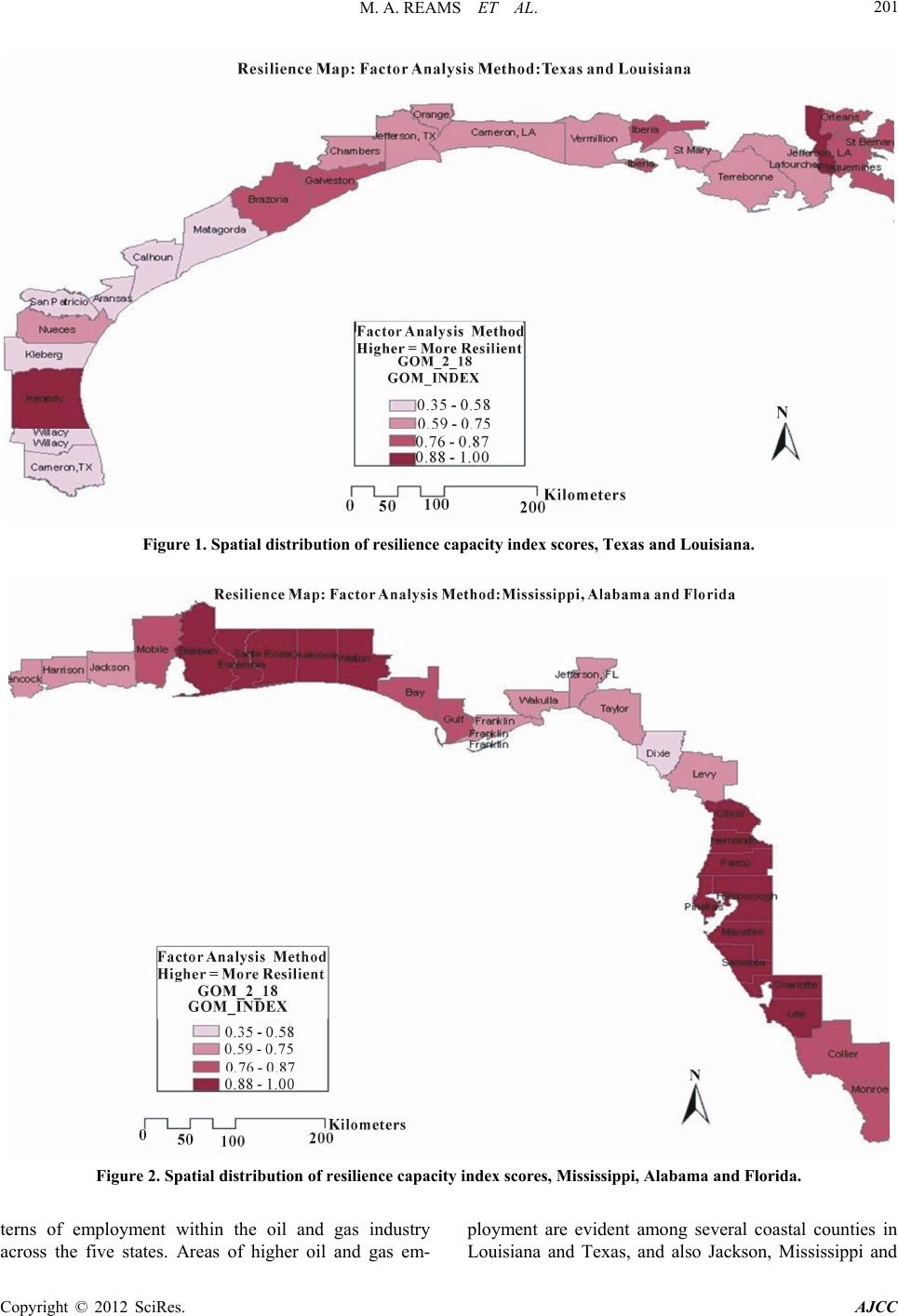

M. A. REAMS ET AL.
201
Figure 1. Spatial distribution of resilience capacity index scores, Texas and Louisiana.
Figure 2. Spatial distribution of resilience capacity index scores, Mississippi, Alabama and Florida.
terns of employment within the oil and gas industry
across the five states. Areas of higher oil and gas em-
ployment are evident among several coastal counties in
Louisiana and Texas, and also Jackson, Mississippi and

M. A. REAMS ET AL.
202
Mobile, Alabama. To determine whether there are statis-
tically significant associations between the presence of
the oil and gas industry and the county-level resilience
scores, we conducted Pearson Correlation Analyses be-
tween variables measuring industry activity and the re-
silience capacity scores for each of the coastal counties in
the study area. The Pearson r Correlation Coefficient ran-
ges from 0 to 1, with values closer to 1 indicating a
stronger association between two variables. The direc-
tional sign of the Pearson r indicates whether the associa-
tion is inverse or positive. Also, the p value determines
whether an observed association is statistically signifi-
cant, with a smaller value (less than 0.10) signaling a
more significant association [28].
We used 2008 employment data from the WholeData
information service, purchased and made available for
this study by the LSU Center for Energy Studies.
WholeData estimated employment figures from County
Business Patterns (CBP) data, using iterative estimation
techniques to fill in the gaps where data may have been
missing in the original CBP data. The employment data
reflects five oil and gas employment categories: NAICS
codes 211 (Oil and Gas Extraction), 213111 (Drilling Oil
and Gas Wells), 213112 (Support Activities for Oil and
Gas), 333132 (Oil and Gas Field Machinery Manufac-
turing), and 541360 (Geophysical Surveying). We used
the sum of employment and establishments for these 5
codes for each county to create two measures of oil and
gas industry presence.
The two counties with the most oil and gas industry
employees are Louisiana’s Terrebonne Parish with 6078
employees, and Nueces County in Texas, with 3420
workers. These counties are followed by several parishes
(counties) in Louisiana: St. Mary Parish (2993), Jefferson
Parish (2540), Orleans Parish (1866), Lafourche Parish
(1491), Iberia Parish (1395), Plaquemine Parish (941);
and two in Texas, Brazoria County (751) and Jefferson
County (517).
We ran bi-variate correlation analyses between the two
measures of oil and gas industry activity (total employ-
ment of the five NAICS categories and number of estab-
lishments) and the resilience capacity scores for the coas-
tal counties within the study area. The analysis examin-
ing the resilience scores for the 52 counties and the oil
and gas activity variables resulted in no statistically sig-
nificant correlations between resilience capacity scores
and industry activity. The resilience-capacity index scores
and total oil and gas industry employment yielded a
Pearson r coefficient of −0.59, p = 0.680. Similarly, the
resilience-capacity index scores and the number of oil
and gas business establishments within a county resulted
in a Pearson r of −0.050 and a p value of 0.756.
6. Conclusions
The study built upon methodology developed by Cutter
and colleagues in their earlier construction of the Social
Vulnerability Index. We included several new variables
drawn from the social-ecological resilience literature that
indicate the capacity for adaptability or resilience. These
include measures of the financial resources and public
investment patterns of local governments, land elevation,
and citizen involvement in public affairs. By combining
these indicators with measures of social vulnerability,
our resilience-capacity index yields useful information
about the relative vulnerabilities and adaptive resources
of these communities. Counties with higher capacities for
resilience include the suburban areas of New Orleans and
Tampa, and the rapidly growing beach tourist communi-
ties of Alabama and Florida. Counties that scored higher
tended to invest more in education, have higher per capi-
ta incomes, more women in the workforce, higher mean
land elevation, more children and higher rates of voter
participation.
The Pearson Correlation Analyses yielded no evidence
of statistically significant associations between the cal-
culated resilience-capacity scores and measures of oil
and gas industry activity within the coastal counties. The
communities located in the area known as the “energy
coast” of Louisiana and Texas, areas with higher em-
ployment in the oil and gas industry, were not found to
have greater capacity for resilience than other counties of
the northern Gulf of Mexico.
The calculation of the resilience-capacity index scores
helps identify sources of community resilience to distur-
bances such as hurricanes and sea level rise. As such, the
analysis demonstrates a useful approach for the more
systematic examination and comparison of factors related
to social vulnerability and capacity for resilience among
coastal communities. Insights into which communities
may be more likely to recover following large-scale
storms, floods and coastal land loss as a result of sea
level rise is useful information for researchers, policy-
makers and residents of coastal communities facing nu-
merous, increasing climate-related hazards.
7. Acknowledgements
This research was supported by a grant from the U.S.
Bureau of Ocean Energy Management (BOEM), Coope-
rative Agreement number M07AC12941 and in part by a
joint grant from the National Science Foundation (NSF)
and the US Department of Agriculture (USDA), Federal
Award Number: USDA 2010-65401-21312.
REFERENCES
[1] S. L. Cutter, B. J. Boruff and W. L. Shirley, “Social Vul-
nerability to Environmental Hazards,” Social Science
Quarterly, Vol. 84, No. 2, 2003, pp. 242-261.

M. A. REAMS ET AL. 203
doi:10.1111/1540-6237.8402002
[2] S. R. Carpenter, C. Folke, M. Scheffer and F. Westley,
“Resilience: Accounting the Non-Computable,” Ecology
and Society, Vol. 14, No. 1, 2009, pp. 13-20.
[3] B. Walker, L. Gunderson, A. Kinzig, C. Folke, S. Carpen-
ter and L. Schultz, “A Handful of Heuristics and Some
Propositions for Understanding Resilience in Social-Eco-
logical Systems,” Ecology and Society, Vol. 11, No. 2,
2006, pp. 10-19.
[4] B. H. Walker, J. M. Anderies, A. P. Kinzing and P. Ryan,
“Exploring Resilience in Socio-Ecological Systems through
Comparative Studies and Theory Development: Introduc-
tion to the Special Issue,” Ecology and Society, Vol. 11,
No. 1, 2006, pp. 12-21.
[5] J. Barnett, S. Lambert and I. Fry, “The Hazards of Indica-
tors: Insights from the Environmental Vulnerability In-
dex,” Annals of the Association of American Geogra-
phers, Vol. 98, No. 1, 2008, pp. 102-119.
doi:10.1080/00045600701734315
[6] N. S. N. Lam, M. Reams, A. Baker, L. De Frank and A.
Martin, “On the Development of a Community Resilience
Index,” Paper Presentation: Annual Meeting of the Asso-
ciation of American Geographers, Las Vegas, 26 March
2009.
[7] W. N. Adger, T. P. Hughes, C. Folke, S. R. Carpenter and
J. Rockstrom, “Social-Ecological Resilience to Coastal
Disasters,” Science, Vol. 309, No. 5737, 2005, p. 1036.
doi:10.1126/science.1112122
[8] J. G. Liu, T. Dietz, S. R. Carpenter, M. Alberti, C. Folke,
E. Moran, A. N. Pell, P. Deadman, T. Kratz, J. Lubchenco,
E. Ostrom, Z. Ouyang, W. Provencher, C. L. Redman, S.
H. Schneider and W. W. Taylor, “Complexity of Coupled
Human and Natural Systems,” Science, Vol. 317, No.
5844, 2007, pp. 1513-1516.
[9] C. S. Holling, “Understanding the Complexity of Eco-
nomic, Ecological, and Social Systems,” Ecosystems, Vol.
4, No. 5, 2001, pp. 390-405.
doi:10.1007/s10021-001-0101-5
[10] C. Folke, S. Carpenter, T. Elmqvist, L. Gunderson C. S.
Holling and B. Walker, “Resilience and Sustainable De-
velopment: Building Adaptive Capacity in a World of
Transformations,” Ambio, Vol. 31, No. 5, 2002, pp. 437-
440.
doi:10.1639/0044-7447(2002)031[0437:RASDBA]2.0.C
O;2
[11] A. K. Ahmed, “Concepts and Practices of Resilience: A
Compilation from Various Secondary Sources,” Working
Paper prepared for the Coastal Community Resilience
(CCR) Program, US Agency for International Develop-
ment, 2006
[12] A. Baker, “Creating an Empirically Derived Community
Resilience Index of the Gulf of Mexico Region,” Master’s
Thesis, Louisiana State University, Baton Rouge, 2009.
[13] W. N. Adger, “Vulnerability,” Global Environmental Chan-
ge, Vol. 16, No. 3, 2006, pp. 268-281.
doi:10.1016/j.gloenvcha.2006.02.006
[14] B. L. Turner, R. E. Kasperson, P. A. Matson, J. J.
McCathy, R. W. Corell, L. Christensen, N. Eckley, J. X.
Kasperson, A. Luers, M. L. Martello, C. Polsky, A. Pul-
sipher and A. Schiller, “Science and Technology for Sus-
tainable Development Special Feature,” Proceedings of
the National Academy of Sciences, Vol. 100, No. 14,
2003, pp. 8074-8079. doi:10.1073/pnas.1231335100
[15] R. E. Kasperson, K. Dow, E. R. M. Archer, D. Caceres, T.
E. Downing, T. Elmqvist, S. Eriksen, C. Folke, G. Han, K.
Iyengar, C. Vogel, C. A. Wilson and G. Ziervogel. “Vul-
nerable Peoples and Places,” In: R. Hassin, R. Scholes
and N. Ash, Eds., Millennium Ecosystem Assessment,
Island Press, Washington, 2005, pp. 145-162.
[16] M. Fordham, “Gender, Disaster and Development: The Ne-
cessity for Integration,” In: M. Pelling, Ed., Natural Dis-
asters and Development in a Globalizing World, Rout-
ledge, London, 2003, pp. 57-74.
[17] A. A. Yusuf and H. Francisco, “Climate Change Vulner-
ability Mapping for Southeast Asia,” Economy and En-
vironment Program for Southeast Asia (EEPSEA), 2009.
http://web.idrc.ca/uploads/user-S/12324196651Mapping_
Report.pdf.
[18] J. MacCarthy, O. Canziani, N. Leary, D. Dokken and K.
White, “Climate Change 2001: Impacts, Adaptation and
Vulnerability,” IPCC (Inter-Governmental Panel on Cli-
mate Change), Cambridge University Press, Cambridge,
2001.
[19] R. Nelson, P. Kokic, S. Crimp, H. Meinke and S. M.
Howden, “The Vulnerability of Australian Rural Commu-
nities to Climate Variability and Change: Part I—Con-
ceptualizing and Measuring Vulnerability,” Environmen-
tal Science & Policy, Vol. 13, No. 1, 2009, pp. 8-17.
doi:10.1016/j.envsci.2009.09.006
[20] R. Nelson, P. Kokic, S. Crimp, P. Martin, H. Meinke, S.
M. Howden, P. de Voil and U. Nidumolu, “The Vulner-
ability of Australian Rural Communities to Climate Vari-
ability and Change: Part II—Integrating Impacts with
Adaptive Capacity,” Environmental Science & Policy,
Vol. 13, No. 1, 2009, pp. 18-37.
doi:10.1016/j.envsci.2009.09.007
[21] F. Ellis, “Rural Livelihoods and Diversity Indeveloping
Countries,” Oxford University Press, Oxford, 2000.
[22] S. L. Cutter and C. T. Emrich, “Moral Hazard, Social
Catastrophe: The Changing Face of Vulnerability along
the Hurricane Coasts,” The Annals of the American
Academy of Political and Social Science, Vol. 604, No. 1,
2006, pp. 102-112. doi:10.1177/0002716205285515
[23] S. Cutter and C. Finch, “Temporal and Spatial Changes in
Social Vulnerability to Natural Hazards,” Proceedings of
the National Academy of Sciences (PNAS), Vol. 105, No.
7, 2008, pp. 2301-2306. doi:10.1073/pnas.0710375105
[24] M. J. Norusis, “SPSS 12.0 Statistical Procedures Com-
panion,” Prentice Hall, Upper Saddle River, 2003.
[25] Louisiana Oil and Gas Association (LOGA), “Oil and
Gas Statistics,” 2008.
http://www.loga.la/oil-gas-statistics.html
[26] C. Folke, T. Hahn, P. Olsson and J. Norberg, “Adaptive
Governance of Social-Ecological Systems,” Annual Re-
view of Environment and Resources, Vol. 30, No. 1, 2005,
pp. 441-473.
doi:10.1146/annurev.energy.30.050504.144511

M. A. REAMS ET AL.
204
[27] D. Austin, B. Carriker, T. McGuire, J. Pratt, T. Priest and
A. G. Pulsipher, “History of the Offshore Oil and Gas
Industry in Southern Louisiana, Interim Report: Volume
I,” Papers on the Evolving Offshore Industry, US De-
partment of the Interior, Minerals Management Service,
Gulf of Mexico OCS Region, New Orleans, 2004.
[28] R. Antonius, “Interpreting Quantitative Data with SPSS,”
Sage Publications, London, 2003.
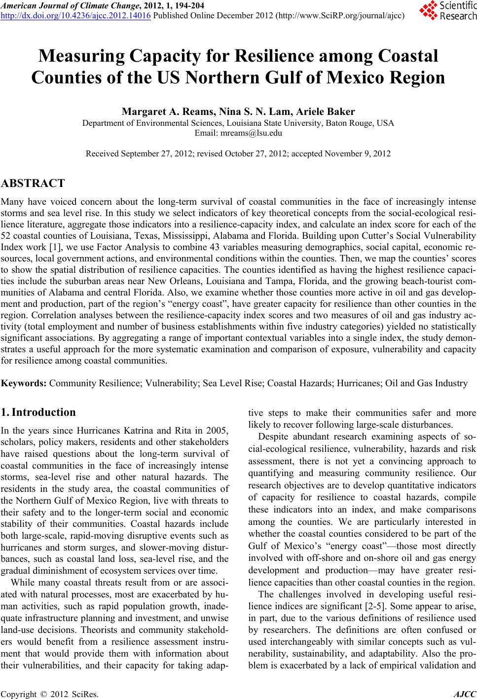