Theoretical Economics Letters, 2012, 2, 557-560
http://dx.doi.org/10.4236/tel.[phone] Published Online December 2012 (http://www.SciRP.org/journal/tel)
Global Relative Prices in the Face of a Pollut ion Transfer
Problem
John Dogbey
Department of Economics, University of Nebraska at Omaha, Omaha, USA
Received September 22, 2012; revised October 23, 2012; accepted November 25, 2012
ABSTRACT
This study focuses on the relationship between trade and relative prices of pollution intensive goods. Seminal to this
idea is the transfer problem. It is based on the idea that environmental quality of two countries that engage in trade
could be affected and this could also have possible environmental quality transfer effects in a third country (geographic
neighbors or trade partners) and a result, terms of trade effects. The paper makes the case that whether the relative price
of a pollutant would suffer during trade will depend on the kind of pollutant it is, distance between the countries in-
volved, countries’ marginal propensity to consume and substitutability of the good. The nature of the pollutant (whether
it is spatially separable in production and or consumption) determines whether it can spillover to trade neighbors or
whether it is transferable to a trade partner with ramifications to its relative price. The paper uses indirect utility func-
tions and compensated demand functions to analyze the terms of trade effects.
Keywords: Relative Prices; Spatially Separable; Trade; Substitutability; Pollutant; Transfers
1. Introduction
The debate on the role of trade in environmental pollu-
tion has attracted a lot of attention in recent years. Many
believe that trade has a debilitating effect on the envi-
ronment and others hold contrary views. For example,
research has been done to determine whether reduction in
trade barriers alters the composition of economic activity,
or leads to a change in the techniques of production and
thus have an effect on the environment. The environ-
mental impacts of trade policies as well the trade impacts
of environmental policies have also been investigated.
These researchers find that trade liberalization may in-
crease specialization in sectors that cause little pollution.
These studies include Grossman and Krueger [1], and
Huang and Labys [2].
The relationship between economic growth and envi-
ronmental pollution has also gained much attention. Re-
searchers find that a liberal trade regime leads to in-
come growth and that economic growth reduces pollu-
tion once a country reaches a certain income threshold.
Other findings are that as trade increases and growth
increases, environmental pollution also increases. The
other side of the coin is that environmental policies
reduce trade and growth. Stricter environmental stan-
dards are also considered necessary for a U-shaped
relationship between pollution and income during
growth as discussed in Grossman and Krueger [1],
Huang and Labys [2], and Grossman and Krueger [3],
and McConnell [4].
On the effect of trade on countries’ Environmental
Kuznets Curve (EKC), a myriad of research has been
carried out. A theoretical work finds that during the tran-
sition from autarky to international trade, the EKC U-
shape relationship may hold for a cross-section of coun-
tries but may not hold for individual economies. The
extent to which consumer preferences and structures
such as education level, sectoral composition of the
economy, and unemployment can spatially and inter-
temporally affect the EKC relationship has been explored
with the result that the level of income at which house-
holds decide to reduce their exposure to pollution de-
pends on the nature of the pollution. For goods that are
spatially separable (i.e., goods which do not generate
pollution during either their production or consumption),
such as SO2 and PM10, there is significant evidence of
such relationship while there is little evidence for non-
spatially separable pollutants such as CO3, O3 and NOx.
Khanna [5], and Khanna and Plassmann [6] document
these views.
Other researchers in the area of welfare and trade ana-
lyze the welfare effects that arise when rich countries
make bilateral or multilateral transfers to poor countries
and conclude that there is a transfer problem in that poor
countries get impoverished when they receive transfers
from rich countries. These researchers include Band-
yopadhay and Majumdar [7], and Bandyopadhyay and
C
opyright © 2012 SciRes. TEL

J. DOGBEY
558
Munemo [8], and Bhagwati, Brecher, and Hatta [9], and
Bhagwati and Brecher [10,11].
While a plethora of literature looks at the link between
trade and the environment, or trade and relative prices,
no research has made the link between pollution, trade
and relative prices. This paper attempts to fill the gap by
providing a comparative statistics analysis to examine
what happens to relative prices during trade when the
good in question is a pollutant. It establishes a relation-
ship between pollution, trade, welfare and relative prices.
Thus, it addresses the issue of global welfare effects or
terms of trade effects when countries engage in trade
involving pollutants. The rest of this paper is organized
as follows: In the next section I present the models and
derive the results, followed by the comparison of the
results and intuition behind them in Section 3, then pre-
sent the concluding remarks and policy recommendations
in Section 4.
2. The Model
2.1. The General Model
This paper uses compensated demand functions, indirect
utility functions and the overspending functions of coun-
tries to analyze bilateral trade in a pollutant in a multilat-
eral context. This model assumes a three-country world:
countries α, γ, β, namely the developed country, the de-
veloping country and the non-participant; only countries
γ and β could be neighbors (the developed country’s aim
is to transfer pollution, so it can only engage in such a
trade with a developing country that is not its neighbor).
The model also assumes a two-good world: Good X and
good Y; good X is the pollutant.
The paper considers three cases of the pollutant and
hence three models. The first two cases relate to a situa-
tion where consumption or production of the good is spa-
tially separable (either consumption or production does
not generate pollution) while the third case relates to a
situation where both production and consumption are
non-spatially separable. Case 1 involves a situation where
only consumption generates pollution (only consumption
is non-spatially separable) and it is assumed that the de-
veloped country transfers pollution by exporting good X
to the developing country. Case 2 is the one in which
only the production of good X generates pollution (only
production is non-spatially separable), and the developed
country is assumed to transfer pollution by exporting
production or the pollution generating activities to the
developing country, γ. Case 3 is a scenario where both
the production and consumption of good X generates
pollution (consumption and production are both non-
spatially separable). The developed country is assumed
to still export production to the developing country, with
the possibility of importing the finished goods, thereby
transferring the production emissions.
The cases above thus result in three models. The over-
spending (indirect utility) function of each country, ,
is its cost (expenditure) less its revenue.
i
c
Let = the relative price of good X;
i
q
i
u
P
= the welfare level of country ; i
= the value (cost) of the pollution in terms of good
Y;

= inverse distance between country β and γ; 0 ≤ δ <
1;


,
ii
equ = the expenditure function of country ; i


i
rq = the revenue function of country ; i


,
i
xqi u = the compensated import-demand function
of good X by country .
i
Then the overspending function in autarky is given by:





1;,,,,.
iiiii
cueurqiqq

 
2.2. Case 1: Only Consumption Generates
Pollution
Introducing trade in good X, the budget equation for each
country will include P (the volume of trade in the pol-
lutant), which will be adding to the benefit (revenue)
component of the developed country (the exporter), but
reducing the revenue component (or adding to the cost
component) of the developing country (importer) and the
non-participant (depending on the distance between the
importer and the non-participant). In other words, the
export of the pollutant reduces the overspending function
of country α but increases the overspending functions of
countries γ and β. The model comprises of the budget
equations of the three countries and the market clearing
equation of good X:


,Pqcu

0 (2.1)


,Pqcu

 0

 (2.2)
2


,Pqcu

0 (2.3)




,,,uuxq xqxqu

0

 (2.4)
3
As the developed and developing country trade the
production and, hence, the consumption of the pollutant
increases (so P increases). Taking total differentials of
Equations (2.1)-(2.4)4 and augmenting gives:
1During trade, a country’s overspending function will increase (de-
crease) if it is importing (exporting) good X.
2The budget equation of the non-participant is affected not by the full
value of the pollution, but by a fraction. The longer the distance be-
tween the non-participant and its neighbor, the smaller the value of δ
and hence the smaller the value of the pollution transfer or spillover.
When δ approaches zero, the non-participant’s overspending function
and budget equation will be the same.
3By Walras Law, the market clearing equation of good Y is omitted.
4Total differential of (2.1) is: , and (2.4) is:
ddd
uq
cu cq P
 
0


dd0
qq
x xqP
 
ddd
uuu q
xu xuxux
  


.

J. DOGBEY 559
100 1
d
010dd
001 1
d
0
d
q
xu
xup
xu
xxxx q























 



where i
qqqq q
x
xxx x

 (2.5)
i
q
i
x
c (2.6)
5
1
i
ii
uu i
c
ce u

 
 (2.7)
Equation (2.7) implies that a country will consume
good X until it reaches a point where the percentage in-
crease in its utility exactly equals the percentage increase
in its cost or expenditure. In Equation (2.5)6, q
x
is the
summation of the substitution effects, which are always
negative for a normal good.
Let Δ be the negative of the slope of the global excess
demand function. This represents the Marshall Lerner
Condition (MLC) and the Walrasian stability implies that
Δ > 07. Thus, where,
0,
qu uu
xxxxx xx
 

0.
q
x
The effect of an increase in P on the relative price of
the good using Cramer’s Rule is:
d0
dΔ
uu u
xx x q
P
 
 
 (2.8)
(2.8) implies that the relative price of good X (when
consumption is non-spatially separable) increases as the
trade in X increases. Note that ,,
uu u
x
xx


represent each
country’s marginal propensity to consume8, which is
always positive for normal goods.
2.3. Case 2: Only Production Generates
Pollution
This is the case where country α exports raw materials to
country γ and or engages in pollution generating active-
ties in it since the production of good X emits pollution
as opposed to its consumption. This model is only an
extension of Case 1 in that an emission tax,
, is applied, which reduces the amount of
pollution generated in country γ and the possible amount
of pollution spillovers in country β.

π0π1

0
The model is as follows:

,Pqcu

 (3.1)




1π0,cu Pq



 (3.2)




1π0,cu Pq


 (3.3)




,0,,cucuqqcuq


 (3.4)
The corresponding augment after taking total differ-
enttials and making similar assumptions as in Case 1 is:


100 1
d
010 1π
dd
0011π
d
0
d
q
xu
xuP
xu
xxxx q
























 


The effect of an increase in P on the relative price of
the good using Cramer’s Rule is:




1π1π
d0
dΔ
uu
xxx
q
P

 
u


 (3.5)
From Equation (3.5) above, it is apparent that the rela-
tive price of the good (when production is non-spatially
separable) falls as trade in the pollutant increases.
2.4. Case 3: Both Consumption and Production
Generate Pollution
This is the case where production and consumption of the
pollutant are non-spatially separable. In this case, the
developed country still shifts production to the develop-
ing country but imports the good for consumption and
hence reduces the total amount of pollution by the pro-
duction emissions. The budget equations are:


,Pqcu

 0 (4.1)




2π0,cu Pq



 (4.2)




2π0,cu Pq


 (4.3)
9




,0,,cucuqqcuq


 (4.4)
The overspending function and the compensated de-
mand functions remains the same as in Cases 1 and 2.
Using the same conditions and assumptions as above and
totally differentiating and augmenting, gives:


100 1
d
010 2π
dd
001 2π
d
0
d
q
xu
xuP
xu
xxxx q






 
















 



5Shephard Lemma.
6This is the substitution effect; it is assumed that X and Y are substi-
tutable in production and consumption.
7The slope of the excess demand function is: qu uu
x
xx xxxx


 The determinant of the above is same as before, and
the effect of an increase in P on the relative price of the

.
The MLC is thus the negative of this and it is positive. See Bhagwati,
Brecher, and Hatta [9].
8The Marginal Propensity to Consume is given by ii i
uu u
x
ex

,since
, from Equation (2.7). 1
i
u
e
9Since the developing country’s production of the pollutant will be
affected by the emission but not consumption its budget equation
is




1π0,qcu PP

,


which simplifies to Equation (4.3).

J. DOGBEY
560
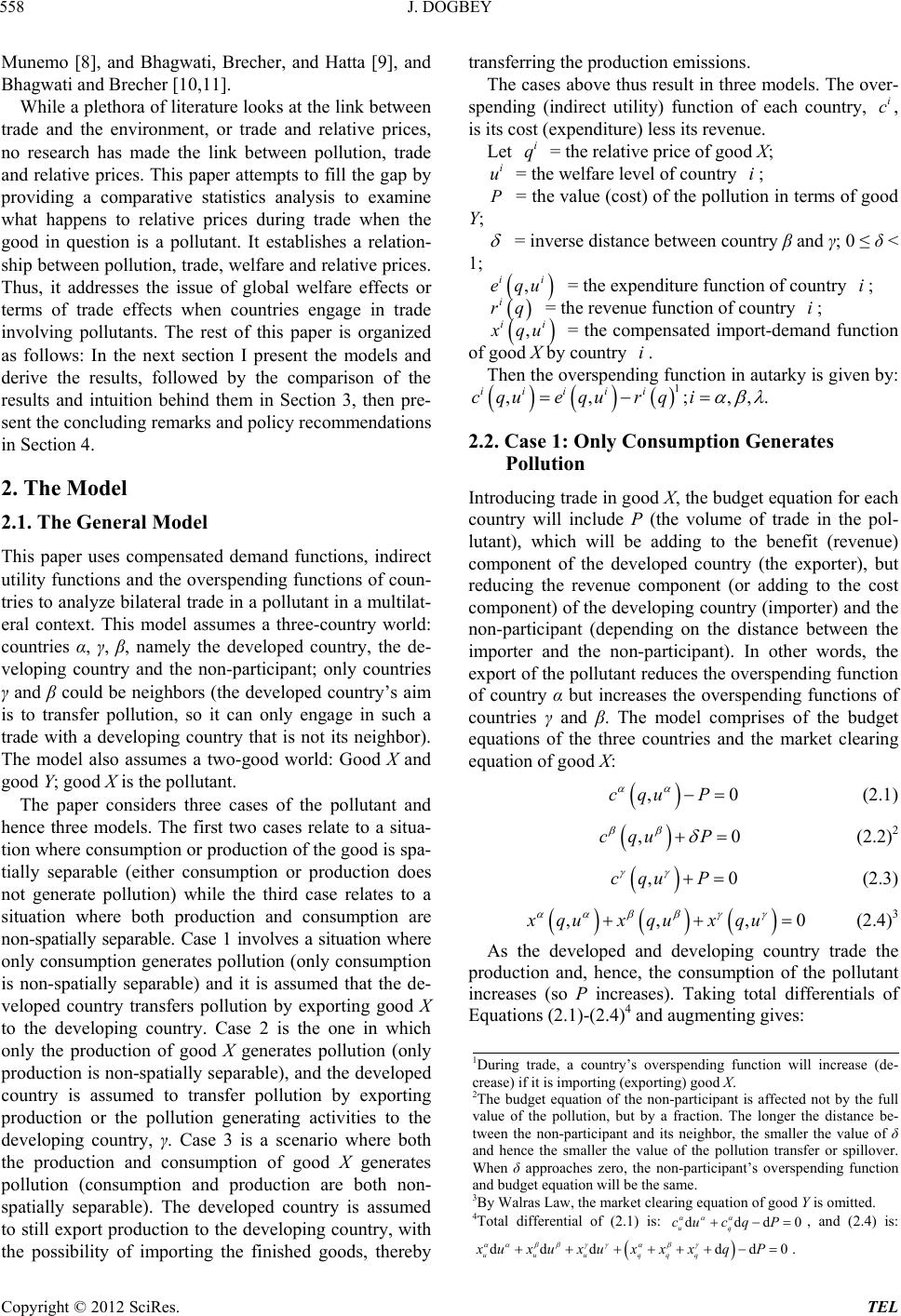
good using Cramer’s Rule is:



2π12π
d0
dΔ
uu
xx
q
P

 
 
u
x

(4.5)
From Equation (4.5) above, it is obvious that the rela-
tive price of the good (when consumption and production
are both non-spatially separable) falls as the pollution
generating activity increases.
3. Comparing Results for All Cases
This section compares the comparative static analysis for
all three cases and provides intuition behind the results
obtained.
If the good is non-spatially separable in consumption
only (Case 1) the relative price of the good increases. If
the good is non-spatially separable in production (Case 2)
or non-spatially separable in both consumption and
production (Case 3) the relative price of the good falls.
Note that even though Cases 2 and 3 have same direction
(sign) for the relative price of the good, the magnitude is
higher for former than the latter case. The results there-
fore indicate that goods that are nonspatially separable in
at least production have relatively lower relative prices.
The intuition behind the above result is that ways of
restraining firms from increasing pollution emissions are
more effective than ways of restraining consumers. Cou-
pled with government regulations, specialization can
enable firms find efficient ways of producing the good in
order to reduce emissions considerably. Lower pollution
levels cost society and firms less and this causes the
global relative price of the good to fall. As there is little
or no specialization in or restraint on consumption, in-
crease trade in goods that are non-spatially separable in
consumption reflects directly in the relative price of the
goods. Second, relatively lower emission tax on firms in
the developing country reduces the cost of production
and hence the fall in the relative price of the good.
4. Concluding Remarks
This study investigates the direction of global relative
prices during bilateral trade involving a pollutant in a
multilateral context. The results suggest that increased
trade in goods that generate pollution in production or in
both production and consumption will reduce relative
prices as opposed to goods that generate pollution in
consumption only. Thus even though a good may be a
pollutant, depending on how spatially separable it is,
trade and specialization can still cause it’s relative price
to fall. This is true for the good in question even in coun-
tries that are non-participants.
REFERENCES
[1] G. Grossman and A. Krueger, “Environmental Impacts of
a North American Free Trade Agreement,” NBER Work-
ing Paper Series, MIT Press, Cambridge, 1991.
[2] H. X. Huang and W. Labys, “Modeling Trade and Envi-
ronmental Linkages in China,” International Journal of
Global Issues, Vol. 4, No. 4, 2004, pp. 242-266.
doi:10.1504/IJGENVI.2004.006053
[3] G. Grossman and A. Krueger, “Economic Growth and the
Environment,” The Quarterly Journal of Economics, Vol.
112, No. 3, 1995, pp. 353-377.
[4] K. E. McConnell, “Income and the Demand for Environ-
mental Quality,” Environment and Development Eco-
nomics, Vol. 2, No. 4, 1997, pp. 383-399.
doi:10.1017/S1355770X9700020X
[5] N. Khanna, “The Income Elasticity of Non-point Source
Air Pollutants: Revisiting the Environmental Kutznets
Curve,” Economic Letters, Vol. 77, No. 3, 2002, pp. 387-
392. doi:10.1016/S0165-1765(02)00153-2
[6] N. Khanna and F. Plassmann, “The Demand for Envi-
ronmental Quality and the Environmental Kuznets Curve
Hypothesis,” Ecological Economics, Vol. 51, No. 3-4,
2004, pp. 225-236.
doi:10.1016/j.ecolecon.2004.06.005
[7] S. Bandyopadhyay and B. Majumdar, “Multilateral Trans-
fers, Export Taxation and Asymmetry,” Journal of De-
velopment Economics, Vol. 73, No. 2, 2004, pp. 715-725.
doi:10.1016/j.jdeveco.2003.05.001
[8] S. Bandyopadhyay and J. Munemo, “Transfers, Trade,
Taxes and Endogenous Capital Flows: With Evidence
from Sub-Saharan Africa,” International Journal of Busi-
ness and Economics, Vol. 5, No. 1, 2006, pp. 29-40.
[9] J. Bhagwati, R. Brecher and T. Hatta, “The General The-
ory of Transfers and Welfare: Bilateral Transfers in a
Multilateral World,” American Economic Review, Vol. 73,
1983, pp. 606-618.
[10] J. Bhagwati and R. Brecher, “Foreign Ownership and the
Theory of Trade and Welfare,” Journal of Political Eco-
nomy, Vol. 89, No. 3, 1981, pp. 497-511.
doi:10.1086/260982
[11] J. Bhagwati and R. Brecher, “Immiserizing Transfers
from Abroad,” Journal of International Economics, Vol.
13, No. 3-4, 1982, pp. 353-364.
doi:10.1016/0022-1996(82)90063-0