J. Serv. Sci. & Management, 2009, 2: 15-28
Published Online March 2009 in SciRes (www.SciRP.org/journal/jssm)
CDS Evaluation Model with Neural Networks
Eliana Angelini
1
, Alessandro Ludovici
1
1
University “G. d’Annunzio” of Pescara, University “G. d’Annunzio” of Pescara
Received May 6
th
, 2008; revised December 27
th
, 2008; accepted February 5
th
, 2009.
ABSTRACT
This paper provides a methodology for valuing credit default swaps (CDS). In these financial instruments a sequence of
payments is promised in return for protection against the credit losses in the event of default. Given the widespread use
of credit default swaps, one major concern is whether the credit risk has been priced accurately. Credit risk assessment
of counterparty is an area of renewed interest due to the present financial crises.
This article proposes a non parametric model for estimating pricing of the CDS, using learning networks, based on
the structural approach pioneered by Merton [1] as regards the independent variables; he proposed a model for as-
sessing the credit risk of a company by characterizing the company’s equity as a call option on its assets. The model
that we are introducing turns out peculiar not only for the use of the neural network, but also for the use of the implied
volatility of one-year options written on the shares of the analyzed companies, instead of historical volatility: this leads to
a higher capability of getting the signals launched by the market about the future creditworthiness of the firm (historic
volatility, being a medium value, brings in temporal lags in the evaluation). Besides, our analysis differs from the
structural approach for the fact that it considers the 30-month mean-reverting historical series for CDS spreads, and this
turns out to be one of the main advantages of our forward-looking model.
Keywords: credit derivatives, CDS, neural networks, pricing models, credit spreads, implied volatility
1. Introduction
In recent years, the market for credit derivatives has ex-
panded dramatically. Credit derivatives are flexible and
efficient instruments that enable users to isolate and trade
credit risk. Credit derivatives allow users to isolate credit
risk from other quantitative and qualitative factors asso-
ciated with owing an exposure. Hence, they can be used
to transfer and hedge credit risk in an efficient and flexi-
ble manner, customized to a client’s requirements. This
transfer of credit risk may be complete or partial, and
may be for the life of the asset or for a shorter period.
Credit risk includes not just default or insolvency risk but
also changes in credit spreads and thereby market values,
changes in credit ratings and generic changes in credit
quality. Credit derivatives can be used when a sale in the
cash market is either not efficient or not possible. Even
when cash market alternatives exist, credit derivatives
may be preferred because they do not require funding.
Furthermore, since derivatives are over-the-counter con-
tracts, transactions are confidential. Finally, speed of set-
tlement and liquidity are reasons why credit derivatives
are a better alternative to the reinsurance market. Credit
derivatives are swaps, forward and option contracts, par-
ticularly credit default swaps (CDS); they can be used to
hedge against all these types of credit risk. For a simple
credit default swap, over some time period, one counter-
party (the protection seller) receives a predetermined fee
payment from another counterparty (the protection buyer);
in return, the protection seller agrees that in the case of a
credit event of a reference entity, it will pay the seller the
loss on a bond of the reference entity, that is the bond’s
par value less its recovery.
Nowadays, banks, corporate, hedge funds, insurance
companies and pension funds are hugely exposed as buy-
ers or sellers, or both. By transferring the risk, the CDS
have acted as a kind of insurance and provided incentives
for risk-taking. They are therefore at the heart of the pre-
sent crisis.
Given the widespread use of credit default swaps, as an
investment or a risk management tool, one major concern
is whether the credit risk has been priced accurately. This
article proposes a non parametric model for estimating
pricing of these credit derivatives, using learning net-
works. The recent application of nonlinear methods, such
as neural networks to credit risk analysis, shows promise
of improving on traditional credit models. Neural net-
works differ from classical credit systems mainly in their
black box nature and because they assume a non-linear
relation among variables. The two main issues to be de-
fined in a neural network application are the network
typology and structure and the learning algorithm. The
connections (links) among neurons have an associated
weight which determines the type and intensity of the
information exchanged. As regards the independent vari-

16 ELIANA ANGELINI, ALESSANDRO LUDOVICI
ables of the model, we start from the typical assumption
of the structural approach based on the theoretical foun-
dation of Merton’s [1] option pricing model: the relevant
information in order to evaluate credit risk can be ob-
tained from the market data of the analyzed companies.
The model developed by Merton views a firm’s equity as
an option on the firm (held by the shareholders) to either
repay the debt of the firm when it is due, or abandon the
firm without paying the obligations. What makes that
model successful is its reliance on the equity market as an
indicator, since it can be argued that the market capitali-
zation of the firm (together with the firm’s liabilities)
reflect the solvency of the firm. Therefore, option pricing
theory is used in order to create a link between the credit
market and the securities market. The model that we are
introducing turns out peculiar not only for the use of
neural networks, but also for the use of the implied vola-
tility of one-year options written on the shares of the
companies, instead of historical volatility: this leads to a
higher capability of getting the signals launched by the
market about the creditworthiness of the firm (historical
volatility, being a medium value, brings in temporal lags in
the evaluation). Besides, our analysis differ from the
structural approach for the fact that it consider the
30-month historical series for CDS spreads, and this turns
out to be one of the main advantage of our forward-
looking model.
The paper is organized as follows. The paper begins,
in Section 1, by stating the implications of credit deriva-
tives in portfolio credit risk management. In Section 2,
we first briefly overview the main principles and charac-
teristics of neural networks, focusing the attention above
all on the concepts that are most useful for the application
to financial instruments; then we describe the pricing
model we developed and tested for credit derivatives.
Section 3 develops the theory underlying our implemen-
tation of Merton’s model. Section 4 describes the data
and we present our results: the effectiveness of neural
network in approximating the evaluation of credit default
swap is illustrated. As regards the sample, it includes 18
American firms, relative to various fields, including fi-
nancial institutions which, operating typically with a high
leverage due both to the activity carried out and to the laws
concerning the capital of banks, usually introduces re-
markable factors of distortion in parametric models. We
shall show that neural networks are not affected by this
problem. The temporal range embraces the period Sep-
tember 2002-March 2006: we have considered the five-
year CDS spread relative to each firm, for a total of 180
observations on a quarterly basis obtained through the
Fitch™ database. As already pointed out, implied volatil-
ity has a determining role among the variables; in fact we
have obtained a positive correlation with CDS spreads
equal to 0.6338. Leverage is another key variable, ob-
tained dividing the face value of the debt of the firm by the
total of its liabilities (including the market capitalization),
getting the data from the Bloomberg™ database. We have
considered the risk free rate equal to one-year constant
maturity Treasury Bills yield, taken from the Federal Re-
serve System database. We then discuss in detail the ex-
perimental settings and the results we obtained, leading to
considerable accuracy in prediction. The architecture of
the neural network is feed-forward, trained for 17000
learning epochs using the back-propagation algorithm,
with two hidden layers of 9 and 10 neurons each: by the
study carried out it turns out obvious that neural networks
are able to totally capture the variability relative to the
market dynamics of credit default swap. The paper ends
evidencing that, as far as this field of the financial markets
is concerned, neural networks constitute a highly valid
instrument of calculation: in fact there still does not exist
in literature a formula of evaluation for the CDS, able to
tie the quoted spreads to the specific underlying variables
of each examined firm, and the neural network can, as will
be shown, satisfy this lack with high effectiveness, facing
the problem of determination of the functional form from a
statistical point of view. As we will show, it is easy to
calculate the sensitivity of the CDS spread to each inde-
pendent variable, in order to determine a statistical pricing
formula for CDS.
The paper concludes with a discussion of advantages
and limitations of the solution achieved.
2. Credit Derivatives: Innovative Financial
Instruments
Credit derivatives are financial instruments used to trans-
fer credit risk of loans and other assets. They are bilateral
financial contracts with payoffs linked to a credit related
event such as a default, credit downgrade or bankruptcy.
There are various types, but the basic structures of all
credit derivatives are swaps, options and forwards. Due to
their high flexibility credit derivatives can be structured
according to the end-users’ needs. For instance, the
transfer of credit risk can be effected to the whole life of
the underlying asset or for a shorter time, and the transfer
can be a complete or a partial one. Delivery can take place
in the form of over the counter contracts or embedded in
notes. Moreover, the underlying can consist of a single
credit-sensitive asset or a pool of credit-sensitive assets [2].
2.1 Credit Derivatives: Products and Structures
The most important and widely used credit derivative is a
credit default swap
1
. It is an agreement in which the one
counterparty (the protection buyer) pays a periodic fee,
typically expressed in fixed basis points on the notional
amount, in return for a contingent payment to the other
counterparty (the protection seller) in the event that a
third-party reference credit defaults. A default is strictly
defined in the contract to include, for example, bankruptcy,
insolvency, and/or payment default. The definition of a
credit event, the relevant obligations and the settlement
mechanism used to determine the contingent payment are
flexible and determined by negotiation between the
1
The credit default swap is also known as credit
default put, credit swap,
default swap, credit put or default put.

ELIANA ANGELINI, ALESSANDRO LUDOVICI 17
counterparties at the inception of the transaction. Since
1991, the International swap and Derivatives association
(ISDA) has made available a standardized letter confir-
mation allowing dealers to transact credit swaps under the
umbrella of an ISDA Master Agreement. The evolution of
increasingly standardized terms in the credit derivatives
market has been a major growth because it has reduced
legal uncertainty that hampered the market’s growth.
The contingent payment in the event of default can be
identified as either:
-a payment of par by the protection seller in exchange
for physical delivery of the defaulted underlying;
-a payment of par less the recovery value of the
underlying as obtained from dealers;
-a payment of a binary, i.e. fixed, amount.
Credit default swaps can be viewed as an insurance
against the default of the underlying or a put option on the
underlying. Figure 1 exhibits the basic structure of a credit
default swap.
Moreover, there is the total return swap, in which one
counterparty (total return payer) pays the other counter-
party (total return receiver) the total return of an asset (the
reference obligation) for receiving a regular floating rate
payment, such as Libor plus a spread. “Total return”
comprises the sum of interest, fees and any change-in
value payments (any appreciation or depreciation) with
respect to the reference obligation.
In contrast to the credit default swap, the total return
swap does not only transfer the credit risk but also the
market risk of the underlying; it effectively creates a
synthetic credit-sensitive instrument. A total return swap
allows an investor to enjoy all of the cash flow benefits of
a security without actually owing the security.
Credit spread option is an option on a reference
credit’s spread in the loan or bond market. In a spread put
option one party pays a premium for the right to sell a
bond to a counterparty at a certain spread at a definite
time in the future. A credit spread option gives the buyer
protection in the event of any unfavourable credit mi-
gration. In a default option, the asset can be put only on
default. The credit spread is the differential yield be-
tween the reference credit and a pre-determined bench-
mark rate. Thus, in credit spread derivatives, payment is
based on the movement of the value of one reference
credit against another.
Figure 1. Credit default swap
that pays out if a specified company’s rating is down-
graded. This kind of option is sometimes embedded in
bond structures.
Finally, credit linked notes are created by embedding
credit derivatives in notes. Credit derivatives have the
advantage that funding is not necessary; whereas credit
linked notes have the benefit of avoiding counterparty risk.
Credit linked notes are frequently issued by special pur-
pose vehicles (corporations or trusts) that hold some form
of collateral securities financed through the issuance of
notes or certificates to the investor. The investor receives a
coupon and par redemption, provided there has been no
credit event of the reference entity. The vehicle enters into
a credit swap with a third party in which it sells default
protection in return for a premium that subsidizes the
coupon to compensate the investor for the reference entity
default risk.
2.2 Fundamental Attractions of Using Credit
Derivatives
In theory, credit derivatives are tools that enable financial
operators to manage their portfolio of credit risks more
efficiently; they enable market participants to devise
flexible personal approaches to the management of credit
risk associated with a variety of underlying financial as-
sets. The promise of these important instruments has not
escaped regulators and policymakers. “Credit derivatives
and other complex financial instruments have contributed
to the development of a far more flexible, efficient, and
hence resilient financial system than existed just a quar-
ter-century ago” [3].
The credit derivatives market offers its users a range of
tools which enable the transfer of credit risk. A brief
review of the available products reveals that in most
cases one party to a transaction receives a fee and com-
mits to provide the other party with a payment should the
credit quality of a third party deteriorate. Whilst the
mechanism contained in these products are easy to un-
derstand, the broad range of applications is not immedi-
ately obvious.
The users of the risk-management benefits of credit
derivatives tend to be quite diverse. An increasingly im-
portant user group includes financial institutions, corpo-
rate and fund managers. Financial institutions have em-
braced the full range of benefits; the use of credit deriva-
tives by banks has been motivated by the desire to improve
portfolio diversification and to improve the management
of credit portfolios. Corporate is also looking to reduce the
credit exposure to key trading partners and specifically
they are interested in using credit derivatives to isolate
credit risks in project financing. For fund managers, al-
though the asset benefits of credit derivatives still suffer
from lack of liquidity, the use of structures that hedge out
spread risk has some appeal.
This paragraph focuses on a range of uses for credit
derivatives and divides them between credit risk man-
agement and asset opportunities
2
[4,5].
2
For more detailed information on the characteristics of credit deriva-
tives see DAS
, S., (1998); TAVAKOLI, J.M., (1998).

18 ELIANA ANGELINI, ALESSANDRO LUDOVICI
2.2.1 Using Credit Derivatives for Managing Credit Risk
The principal feature of these instruments is that they
separate and isolate credit risk facilitating the trading of
credit risk with the purpose of:
-replicating credit risk;
-transferring credit risk;
-hedging credit risk.
In practice, the rationale behind a transaction may relate
to the management of credit lines, to regulatory capital
offsets, to balance sheet optimization, portfolio hedging
and diversification or pure risk reduction itself. Credit
derivatives can be used as a risk management tool by
portfolio managers to:
-Achieve portfolio diversification: credit derivatives
can be used to achieve portfolio diversification by
allowing access to previously unavailable credits.
They can also be used to diversify across a range of
borrowers and to gain exposure to an asset without
owing it.
-Reduce concentration risk: investors can reduce
portfolio credit risk concentrations using derivatives
structures; they can thus manage country and industry
risks. Reducing credit concentration in loan portfolios
is commonly viewed as the main use of credit
derivatives. However, to date credit derivatives are
generally referenced to assets which are widely traded,
i.e. for which market prices are readily available, or for
which a rating by an international agency is at hand.
-Manage exposures while maintaining client relation-
ships. Changes to credit risk management in the
banking sector are an additional factor contributing to
greater use of credit derivatives. Investors can use
credit derivatives to reduce exposures without selling
them. This effectively frees up credit lines, allowing
more business to be done with a customer.
Furthermore, a bank that is concerned about credit
loss on a particular loan can protect itself by
transferring the risk to someone else while keeping
the loan on its books. As part of their credit risk
management, banks are viewing credit derivatives
more and more often as tradable products, which can
be transferred to third parties before the maturity date
[6,7,8].
-Manage regulatory capital: the new supervisory rules
provided for by Basel II are also increasing the
incentives for banks to use credit derivatives. Where
guarantees or credit derivatives are direct, explicit,
irrevocable and unconditional, and supervisors are
satisfied that banks fulfil certain minimum
operational conditions relating to risk management
processes, they may allow banks to take account of
such credit protection in calculating capital
requirements. A guarantee or credit derivative must
represent a direct claim on the protection provider
and must be explicitly referenced to specific
exposures or a pool of exposures, so that the extent of
the cover is clearly defined and incontrovertible.
Other than non-payment by a protection purchaser of
money due in respect of the credit protection contract
it must be irrevocable; there must be no clause in the
contract that would allow the protection provider
unilaterally to cancel the credit cover or that would
increase the effective cost of cover as a result of
deteriorating credit quality in the hedged exposure. It
must also be unconditional; there should be no clause
in the protection contract outside the direct control of
the bank that could prevent the protection provider
from being obliged to pay out in a timely manner in
the event that the original counterparty fails to make
the payment due. There are cases where a bank
obtains credit protection for a basket of reference
names and where the first default among the
reference names triggers the credit protection and the
credit event also terminates the contract. In this case,
the bank may recognise regulatory capital relief for
the asset within the basket with the lowest
risk-weighted amount, but only if the notional amount
is less than or equal to the notional amount of the
credit derivative. In the case where the second default
among the assets within the basket triggers the credit
protection, the bank obtaining credit protection
through such a product will only be able to recognise
any capital relief if first-default-protection has also be
obtained or when one of the assets within the basket
has already defaulted [9].
2.2.2 Asset Opportunities
Credit derivatives have evolved to become an important
financial asset class. As already argued, credit derivatives
enable credit risk to be separated from the funding com-
ponent of its underlying instrument; as it is often the form
of the underlying instrument that creates obstacles for the
investor, this separation of the credit risk creates important
opportunities. The decision to use the asset opportunities
of credit derivatives tends to be based on one of the fol-
lowing needs:
-Access to new markets: investors can create new
assets with a specific maturity not currently available
in the market;
-Obtain tailored investments: credit derivatives can be
used to create instruments with exact risk- return
profile sought. Maintaining diversity in credit
portfolios can be challenging. This is particularly true
when the portfolio manager has to submit with
constraints such as currency denominations, listing
considerations or maximum or minimum portfolio
duration. Credit derivatives are being used to address
this problem by providing tailored exposure to credits
that are not otherwise available in the wished form or
not available at all in the cash market.
-Improve the risk-return profile of portfolios: credit
derivatives offer new possibilities of turning a given
market opinion into an investment strategy. This
particularly entails assumption of specific types of

ELIANA ANGELINI, ALESSANDRO LUDOVICI 19
credit risk without the acquisition of the asset itself.
Instead of purchasing a specific bond, a market
participant who considers some credit risks to be
overvalued can earn an attractive premium as a
protection seller in the credit default swap market.
Premiums are generated without having to tie up any
capital for the purchase of a bond issue (at least as long
as no credit event occurs). On the other hand, market
participants who consider risks to be underestimated
can purchase protection by paying a premium. Owing
to the limited possibilities for short sales in the bond
market, hedge funds are increasingly entering into
positions in credit derivative market to implement
their financial strategies. In particular:
- to hedge dynamic risks: exposures that change
with market movements can be hedged using credit
derivatives;
- to manage illiquid credits: credit derivatives can be
utilized to actively manage risk in large illiquid loans
portfolios;
- to execute short credit positions: credit derivatives
can be employed to execute short credit positions
without the risk of a short squeeze or high financing
costs. Hence, investors can use them to hedge or take
advantage of deteriorating credit qualities;
- to hedge declining credit quality: default and spread
options and swaps can be used to hedge failing credit
qualities. Credit spread options and swaps can be
used to hedge fluctuations in credit spreads without
having to wait for default to get a payout.
3. The Neural Network Model
The general structure of a neural network model consists
of simple processing units called nodes that interact with
each other using weighted connections. Each unit (node)
receives and processes inputs, and delivers a single out-
put. The input can be raw or output of other processing
units. The output can be the final product or an input to
another unit. In processing the inputs, the model assigns a
weight to each input, where weights represent the relative
strength or importance of inputs. A neural net essentially
represents a nonlinear discriminant function as a pattern
of connections between its processing units.
Neural networks have been used in different fields of
study, such as engineering, medicine, physics and others.
Although the relative structures differ remarkably with
one another, it is possible to point out some fundamental
principles regarding essentially the functioning of such
operative instruments. Moreover, it is important to start
the treatment emphasizing that, in order to analyze the
financial dynamics, relatively little complex networks are
effective, at least compared to those of other fields
3
[10,11,12].
Neural networks offer several advantages over the tra-
ditional statistical methods. First, neural networks do not
require the restrictive assumptions imposed by conven-
tional methodologies. Second, neural networks can de-
velop input-output map boundaries that are highly non
linear
4
[13,14]. Third, they have greater fault tolerance
and adaptability. Neural network examines all informa-
tion available and it can incorporate the new information
into the analysis promptly through its memorization of
previous learning; it updates its weighting scheme so that
it continually “learns” from experience. Thus, neural net-
works are flexible, adaptable systems that can in corpo-
rate changing conditions.
3.1 Architecture of Neural Networks
A neural network relates a set of input variables {x
i
},
i=1,2,..k to a set of one or more output variables {y
j
},
j=1,2,..h. An essential characteristic of a neural network,
differently from other methods of approximation, is that
it uses one or more hidden layers, in which the input
variables are transformed by a logistic or logsigmoid
function: this characteristic, as shown later, gives to these
instruments a particular efficiency in modeling nonlinear
statistical processes.
In the feed-forward neural network parallel elaboration
is associated to the typical sequential elaboration of the
linear methods of approximation. In fact while in the se-
quential elaboration particular weights are given to the
input variables through the neurons of the input layer, in
the parallel one the neurons of the hidden layer operate
further transformations in order to improve the predictions.
The connectors (between the input neurons and the neu-
rons in the hidden layers, and between these and the output
neurons) are called synapses. The feed-forward neural
network with a single hidden layer is the simplest and at
the same time the most used network in the economic and
financial field.
Therefore the neurons process the input variables in two
ways: firstly forming linear combinations and lastly
transforming these combinations through a particular
function, typically the logsigmoid function, illustrated in
Figure 2. Logsigmoid function
3
DOLCINO, F., GIANNINI, C., ROSSI, E., (1998).
For a useful
description of the phenomenon in general terms, see
FLOREANO, D.,
NOLFI, S
., (1993) and GORI, M., (2003).
4
Such feature is important for financial analysis because several studies
have shown that the relation between default risk and financial factor
(variables) are often non linear. See WU and YU (1996); WU (1991).
1
0.9
0.8
0.7
0.6
0.5
0.4
0.3
0.3
0.2
0.1
-
4
-
2 0 2 4

20 ELIANA ANGELINI, ALESSANDRO LUDOVICI
Figure 2. An essential characteristic of this function is
the threshold behavior near values 0 and 1, which turns
out to be particularly suitable to economic problems,
which usually, for very high (or very low) values of the
independent variables, show little changes in response to
small changes of the variables. At the analytical level,
the neural network can be described by the following
equations [15]:
∑
=
+=
m
itiikktk
xn
1,,0,,
ωω (1)
tk
n
tktk
e
nLN
,
1
1
)(
,, −
+
== (2)
∑
=
+=
q
ktkkt
Ny
1,0
γγ (3)
where L(n
k,t
) represents the logsigmoid activation function.
It is a system with m input variables x
i
and q neurons. A
linear combination of these input variables, observed at
time t, with the weights of the input neurons ω
k,i
and the
constant term (bias) ω
k,0
forms the variable n
k,t
. Then this
variable is transformed by the logistic function and be-
comes the neuron N
k,t
at time or observation t. The set of q
neurons at time or observation t is therefore linearly
combined with the coefficient vector k and added to the
constant term ω
k,0
in order to obtain the output y
t
con-
cerning time or observation t, representing the prediction
of the neural network for the analyzed variable. The feed
forward neural network used with the logsigmoid activa-
tion function is often called multi-layer preceptor or MLP
network. A highly complex problem could be treated
widening this structure, and therefore using two (respec-
tively N and P) or more hidden layers [15]:
∑
=
+=
m
itiikktk
xn
1,,0,,
ωω (4)
tk
n
tktk
e
nLN
,
1
1
)(
,, −
+
== (5)
∑
=
+=
s
ktkklltl
N
1,,0,,
ρρρ (6)
tl
p
tl
e
,
1
1
,−
+
= ρ (7)
∑
=
+=
q
ltllt
Py
1,0
γγ (8)
Adding another hidden layer increases the number of
parameters (weights) to be estimated by the factor (s+1)
(q-1)+(q+1), since the net with a single hidden layer, with
m input variables and s neurons has (m+1)s+(s+1) pa-
rameters, while the same net with two hidden layers and q
neurons in the second hidden layer has (m+1)s+(s+1)q+
(q+1) parameters. However the disadvantage of these
models for complexity does not consist of the number of
parameters, which in any case use up degrees of freedom if
the sample size is limited and requires a longer training
time, but of the greater probability that the net converges
to a local rather than global optimum. Anyway it has been
demonstrated that a neural network with two layers is able
to approximate any nonlinear function [16]. A further
quality of this instrument consists exactly of the fact that it
does not just approximate a phenomenon on the basis of a
presumed functional form to be adapted, but at the same
time it determines the functional form and proceeds to the
evaluation of the weights.
In Figure 3 a net with a multiple number of output
variables is illustrated. A neural network with a hidden
layer and two output variables is described by the fol-
lowing equations:
∑
=
+=
m
itiikktk
xn
1,,0,,
ωω (9)
tk
n
tktk
e
nLN
,
1
1
)(
,,−
+
== (10)
∑
=
+=
q
ktkkt
Ny
1,,10,1,1
γγ (11)
∑
=
+=
q
ktkkt
Ny
1,,20,2,2
γγ (12)
It is possible to observe that adding an output variable
implies the evaluation of (q+1) parameters more, equal to
the number of neurons of the hidden layer increased of one
unit. Therefore adding an output variable implies an in-
creasing number of parameters to be estimated, equal to
the number of the neurons of the hidden layer, not to the
input variables. Using a neural network with multiple
outputs makes sense only if these are closely correlated to
the same set of input variables: as an example we could
mention the temporal structure of the rates of inflation or
of the rates of interest. One of the most common criticisms
made to these instruments is that they are substantially
black boxes: questions regarding the nature of the pa-
rameters, the reasons of the choice of their number, of
Figure 3. Neural network with one hidden layer and two
output neurons

ELIANA ANGELINI, ALESSANDRO LUDOVICI 21
the number of the neurons, of the number of the hidden
layers, the reasons that relate the architecture of the net to
the structure of the underlying problem to be explained do
not find an answer.
The risk, when models are based on a high number of
parameters, is that their extreme flexibility [17], being
able to explain anything and its opposite, ends up in not
carrying any knowledge contribution. However, we must
underline that the same criticism can be made to any sta-
tistical approximation method: therefore not only to neu-
ral networks, but also to linear models, univariate and
multivariate regression and so on. Neural networks, in
particular, are able to explain very irregular processes, on
which it is therefore difficult to identify a precise relation
of cause-effect. Therefore the black box criticism consti-
tutes, paradoxically, also one of the greatest qualities of
neural networks. In any case, the simplicity with which it
is possible to increase the number of the parameters of
the net must never make forget the importance, in any
model, of the clarity of the assumptions.
3.2 Data Scaling
A neural network is not able to analyze data or to give
solutions in absolute value: especially if there are data
of an unusually elevated or reduced value, problems of
overflow or underflow could happen. When instead sig-
moid functions are used, it becomes indispensable to
preprocess data: this family of functions in fact has a
codominy of type [0,1] (or [-1,1] in the case of the log-
sigmoid function), for which the values must be scaled
to these intervals otherwise the output of the net would
become useless, being equal to the superior or inferior
threshold in correspondence of all the different values
higher or lower than a determined limit. In other words,
for a great amount of data not standardize to the interval
the neurons would simply transmit the threshold value,
so a wide part of the information would be lost. As far
as the methods, the linear reduction transforms the se-
ries of values x
k
in the series
k
ˆ
x
x
k
, using the following
formulas:
)min()max(
)min(
ˆ
,
,kk
ktk
tk
xx
xx
x−
−
= (13)
if the range is between 0 and 1, and
1
)min()max(
)min(
2
ˆ
,
,
−
−
−
=
kk
ktk
tk
xx
xx
x (14)
if the desired range is between -1 and 1, while the loga-
rithmic reduction uses the formula:
))log(max(
)1log(
ˆ
,
,k
tk
tk
x
x
x+ = (15)
3.3 Learning Process
After the data have been scaled, we have to deal with the
problem of the evaluation of the parameters (weights)
through the process known as learning (training) of the
neural network. Certainly it is a much more complex
problem than the evaluation of the parameters of a linear
model, as for the nature of high nonlinear complexity of
neural networks. For these reasons numerous optimal
solutions can exist, but they do not minimize the differ-
ence between the predictions of the net and the effective
values to be evaluated. In short, in any non linear model
it is necessary to begin the evaluation of the parameters
on the basis of conditions which represent a guess of the
value of the same. However, as it will be shown, the ca-
pability of the process of evaluation of the parameters to
converge to a global optimum depends on the goodness
of these initial hypothesis: in fact if it is situated near a
local optimum instead of the global one [10], it is likely
that the first one will be reached.
This is illustrated in Figure 3: the initial guess of the
parameters (or weights of the neurons) could accidentally
be situated wherever on the x-axis: if it is near a local
minimum, the training process of the net would lead to-
wards this. Later on, it will be observed that the training
process of the network is completed when a point is
reached in which the derivative of the loss function is
null: we must remember that this condition, beyond the
global optimum, identifies also the local ones and the
saddle points. So it can be anticipated that if the learning
coefficient, which indicates the sensibility of the net to
the training process, is too low, this would lead to the
impossibility of the network to escape from local opti-
mums; while if it is too high, it could carry the training
process to oscillate continuously far away from the opti-
mum point, and therefore the network would diverge. In
analytical terms, it is possible to illustrate the learning
process of a net with two hidden layers, for which it is
therefore necessary to determine the set of parameters
Ω={ω
k,i
, ρ
l,k
,γ
l
}.
The problem consists of [18] the minimizing of the loss
function, defined as the sum of the squares of the differ-
ences between the observed data sample y and the predic-
tion of the net ŷ:
Figure 4. Example of succession of local and global mini-
mums
Ω
ψ

22 ELIANA ANGELINI, ALESSANDRO LUDOVICI
∑
=
Ω
−=Ω
T
ttt
yy
1
2
)(
)
ˆ
()(min ψ (16)
);(
ˆΩ=
tt
xfy (17)
in which T is the number of the observations of the out-
put vector y, and f (x
t
;Ω) represents the neural network. Ψ
is a nonlinear function of Ω. All nonlinear optimizations
begin with an initial guess about the solution and try fur-
ther, better solutions until finding the best possible within
a reasonable number of iterations. Different methodolo-
gies have been proposed in order to lead this search:
some make reference to complex results of logical- nu-
merical analysis, e.g. genetic algorithms, in alternative to
the classic method of the reduction of the gradient or
Newton-Raphson method. In any case the chosen algo-
rithm continues until the last iteration n, or in alternative
a tolerance criterion can be set up, stopping the iterations
when the reduction of the error function comes down a
predefined tolerance value. In order to avoid local opti-
mums, a solution could be to determine a first conver-
gence of the process, and then to repeat it with a set of
different initial parameters in order to verify whether the
solution changes. Alternatively, numerous processes
could be carried out to determine the best solution.
However, there are the most important problems when
the number of the parameters increases or the architecture
of the network becomes particularly complex. Paul John
Werbos proposed in the beginning of 1970’s an alterna-
tive to the gradient method called back-propagation
method. It is a very flexible method to avoid the prob-
lems caused by the evaluation of the Hessian matrix in
the reduction of the gradient, and surely it is the most
used method. In the passage from an iteration to the suc-
cessive one in the process of evaluation of the parameters,
the inverse Hessian matrix is in fact replaced by an iden-
tity matrix having dimension equal to the number k of the
parameters, multiplied by the learning coefficient ρ:
00
1
001
)( ZZH ρ −=−=Ω−Ω
−
(18)
In order to avoid oscillations this coefficient is chosen
in the range [0.05,0.5] and it can also be endogenous, that
is it can assume various values when the gradient comes
down and the process seems to converge; or finally dif-
ferent coefficients for the various parameters can be
adopted. However, the problem of the choice of this co-
efficient remains, together with the existence of local
minimums. Moreover, low values of the learning coeffi-
cient, although as anticipated are able to avoid oscilla-
tions, can extend uselessly the convergence of the mini-
mizing process. This can however be accelerated adding
a ‘momentum’ for which at iteration n we will have:
)()(2111 −−−− Ω−Ω+−=Ω−Ω nnnnn Z µρ (19)
Therefore, with µ generally equal to 0.9, the calcula-
tion of the parameters moves more fast outside a plateau
in the error surface. Now we will briefly discuss the
methods used to estimate the effectiveness of the output
of the net. Relatively to the evaluation of the goodness of
the predictions of the net, the most common index is
R-squared (goodness of fit) especially as far as the capa-
bility of the net to predict the data with which it has been
trained is concerned, and the root mean squared error
(Rmse) as for the capability to generalize the predictions
outside the data sample used for the training; in other
words, divided the sample into two parts, the first (in
sample) will be used in order to train the net, and the
other (out of sample), in general equal to about 25% of
total data, will be used to estimate the capability of the
net to predict data coming from the same population but
not used for the training.
However, as to the total amount of necessary data
5
[10],
undoubtedly a neural network requires the evaluation of
many more coefficients than, for example, a linear model,
and this leads to the necessity of a wide sample. Surely
the availability of wide samples improves the predictive
abilities of the net, but it also implies longer training
times. Moreover, the availability of a wide sample not
always is a positive aspect, especially in the financial
field where using very old data brings distortions in the
models, because they tend to vary with extreme rapidity
and therefore very remote data are no more in any rela-
tions with the present ones.
4. Credit Risk Approach: Our Assumptions
The recent history of financial markets shows how, to the
impetuous development of the financial innovation proc-
ess, which has invested all the structural components of
the same, has been associated the constant engagement of
the operators in finding more efficient computational
methodologies, able to be an effective dynamic support
of the analysis. Growing concerns about credit risk have
created the need for sophisticated credit risk analysis and
management tools. Credit risk measurement models and
credit risk management tools are both of significant im-
portance in the credit market.
The valuation of credit default swap depends on the
credit quality of the reference entity. The default predic-
tion has long been an important and widely studied topic.
There are two main types of models that attempt to de-
scribe default processes in the credit risk literature:
structural and reduced form models. The first approach is
based on modeling the underlying dynamics of interest
rates and firm characteristics and deriving the default
probability based on these dynamics
6
[1,19,20,21]. So
they use the evolution of firms’ structural variables, such
as asset and debt values, to determine the time of default.
Merton’s Model was the first modern model of default
and is considered the first structural model. In Merton’s
model, a firm defaults if, at the time of servicing the debt,
its assets are below its outstanding debt. In the second
5
F. Dolcino, C. Giannini, and E. Rossi
, where the concepts of
“evaluation error” and “approximation error” are analyzed, 1998.
6
R. C. Merton, 1974; F. Black and J. COX, 1976; F. A. Longstaff and
E. Schwartz, 1995; H. E. Lelan and K. B. Toft, 1996; C. Dufresne and R
.
Goldstein, 2001.

ELIANA ANGELINI, ALESSANDRO LUDOVICI 23
approach, instead of modeling the relationship of default
with the features of a firm, this relationship is learned from
the data. Reduced form models do not consider the rela-
tion between default and firm value in an explicit manner
[22,23,24]. The time of default in intensity models is the
first jump of an exogenously given jump process. The
parameters governing the default hazard rate are inferred
from market data. Structural default models provide a
link between the credit quality of a firm and the firm’s
economic and financial conditions. Thus, defaults are
endogenously generated within the model instead of
exogenously given as in the reduced approach.
The focus of our model is on the structural approach,
pioneered by Merton, with some important integration.
4.1 A Brief Review of the Structural Approach:
Merton’s Model
Merton proposes a simple model of the firm that provides
a way of relating credit risk to the capital structure of the
firm. The firm has issued two classes of securities: equity
and debt. The equity receives no dividends. The debt is a
pure discount bond. The value of the firm’s assets is as-
sumed to obey a lognormal diffusion process with a con-
stant volatility. Merton adopts are the inexistence of
transaction costs, bankruptcy costs, taxes or problems
with indivisibilities of assets; continuous time trading;
unrestricted borrowing and lending at a constant interest
rate r; no restrictions on the short selling of the assets; the
value of the firm is invariant under changes in its capital
structure (Modigliani-Miller Theorem) and that the firm’s
asset value follows a diffusion process.
Merton models equity in this levered firm as a call op-
tion on the firm’s assets with a strike price equal to the
debt repayment amount (D). If at expiration (coinciding
to the maturity of the firm’s short-term liabilities, as-
sumed to be composed of pure discount debt instruments)
the market value of the firm’s assets (V) exceeds the
value of its debt, the firm’s shareholders will exercise the
option to “repurchase” the company’s assets by repaying
the debt. However, if the market value of the firm’s as-
sets falls below the value of its debt (V<D), the option
will expire unexercised and the firm’s shareholders will
default. The probability of default (PD) until expiration is
set equal to the maturity date of the firm’s pure discount
debt, typically assumed to be one year. Thus, the Pd until
expiration is equal to the likelihood that the option will
expire out of the money. To determine the PD, the call
option can be valued using an iterative method to esti-
mate the unobserved variables that determine the value of
the equity call option, in particular, V (the market value
of assets) and σ
V
(the volatility of assets). These values
for V and σ
V
are then combined with the amount of debt
liabilities D that have to be repaid at a given credit hori-
zon in order to calculate the firm’s distance to default,
defined to be: (V-D)/ σ
V
or the number of standard devia-
tions between current asset values and the debt repay-
ment amount. The higher the distance to default (denoted
DD), the lower the PD. To convert the DD into a PD es-
timate, Merton assumes that asset values are log-nor-
mally distributed.
Define E as the value of the firm’s equity and V as the
value of its assets. Let E
0
and V
0
be the values of E and V
today; in the Merton framework we have:
)()(
2100
dNDedNVE
rt−
−=
T
TrDV
d
V
V
σ
σ )2/()/ln(
2
0
1
++
=
Tdd
V
σ −=
12
where σ
V
is the volatility of the asset value and r is the
risk free rate of interest, both of which are assumed to be
constant. Define D* = De
-rt
as the present value of the
promised debt payment and let L=D* /V
0
be a measure of
leverage. Because the equity value is a function of the
asset value we can use Ito’s lemma to determine the instan-
taneous volatility of the equity from the asset volatility:
00
V
V
E
E
VE
∂
∂
∂
= σ
)(
1
dN
V
E=
∂
∂
where σ
E
is the instantaneous volatility of the company’s
equity at time zero. These equations allow V
0
and σ
V
to
be obtained from E
0
, σ
E
, L and T. The risk neutral prob-
ability, P, that the company will default by time T is the
probability that shareholders will not exercise their call
option to buy the assets of the company for D at the time
T. This depends only on the leverage, L, the asset vola-
tility, σ, and the time of repayment T.
4.2 CDS Valuation
In our analysis, we present some extensions because the
model needs to make the necessary assumptions to adapt
the dynamics of the firm’s asset value process.
We suggest a new way of implementing Merton’s
model using implied volatility, instead of historical vola-
tility: this leads to a higher capability of getting the signals
launched by the market about the creditworthiness of the
firm. The historical volatility is the realized volatility of a
financial instrument over a given time period. Generally,
this measure is calculated by determining the average
deviation from the average price of a financial instrument
in the given time period. Standard deviation is the most
common but not the only way to calculate historical vola-
tility. By definition, historical volatility will always be
backward looking and lag the real-time volatility envi-
ronment. In the current market environment, however,
where both stocks and implied volatility measures are
rising, many measures of historical volatility begin to
seem no more useful.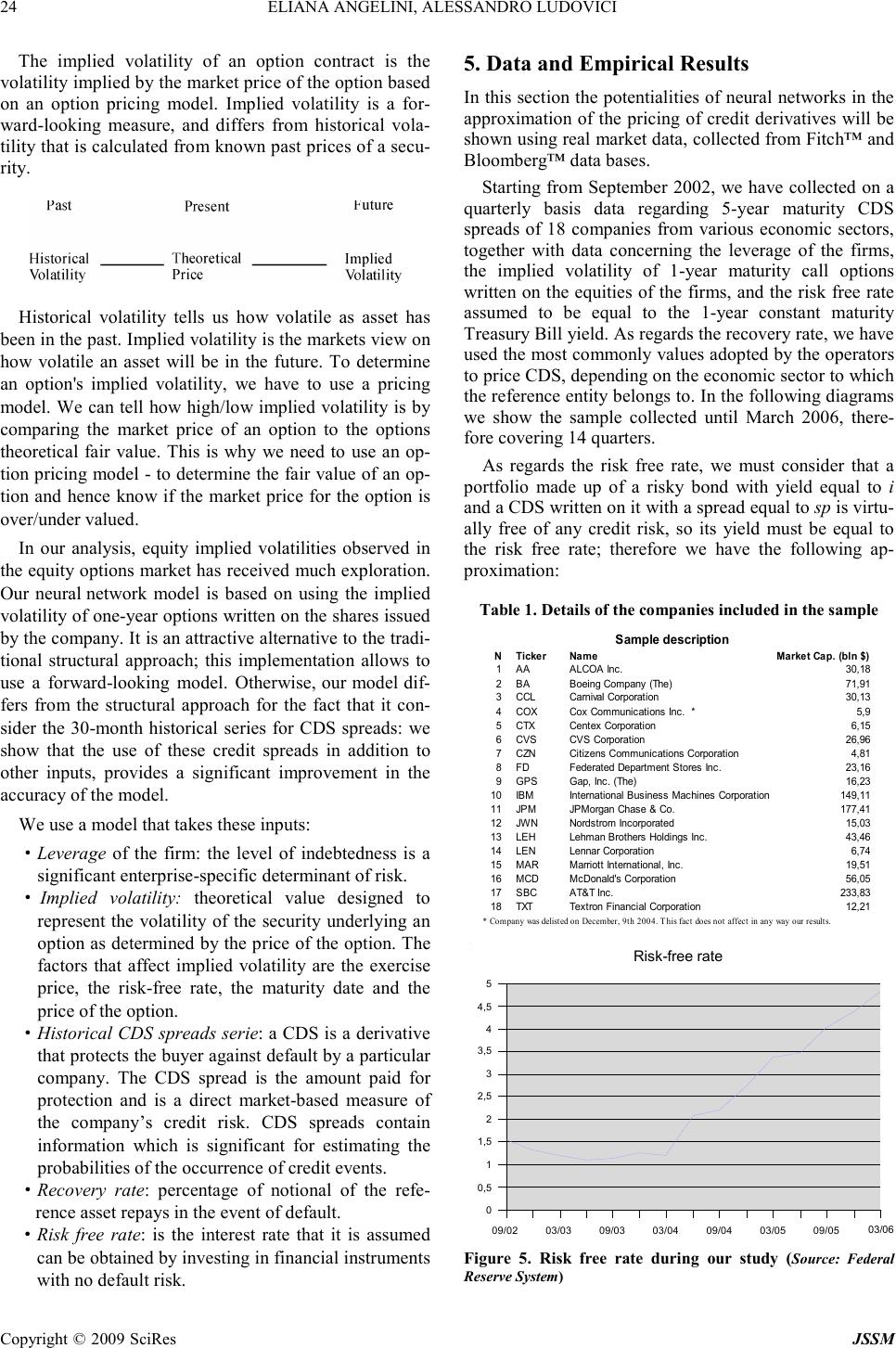

24 ELIANA ANGELINI, ALESSANDRO LUDOVICI
The implied volatility of an option contract is the
volatility implied by the market price of the option based
on an option pricing model. Implied volatility is a for-
ward-looking measure, and differs from historical vola-
tility that is calculated from known past prices of a secu-
rity.
Historical volatility tells us how volatile as asset has
been in the past. Implied volatility is the markets view on
how volatile an asset will be in the future. To determine
an option's implied volatility, we have to use a pricing
model. We can tell how high/low implied volatility is by
comparing the market price of an option to the options
theoretical fair value. This is why we need to use an op-
tion pricing model - to determine the fair value of an op-
tion and hence know if the market price for the option is
over/under valued.
In our analysis, equity implied volatilities observed in
the equity options market has received much exploration.
Our neural network model is based on using the implied
volatility of one-year options written on the shares issued
by the company. It is an attractive alternative to the tradi-
tional structural approach; this implementation allows to
use a forward-looking model. Otherwise, our model dif-
fers from the structural approach for the fact that it con-
sider the 30-month historical series for CDS spreads: we
show that the use of these credit spreads in addition to
other inputs, provides a significant improvement in the
accuracy of the model.
We use a model that takes these inputs:
·Leverage of the firm: the level of indebtedness is a
significant enterprise-specific determinant of risk.
·Implied volatility: theoretical value designed to
represent the volatility of the security underlying an
option as determined by the price of the option. The
factors that affect implied volatility are the exercise
price, the risk-free rate, the maturity date and the
price of the option.
·Historical CDS spreads serie: a CDS is a derivative
that protects the buyer against default by a particular
company. The CDS spread is the amount paid for
protection and is a direct market-based measure of
the company’s credit risk. CDS spreads contain
information which is significant for estimating the
probabilities of the occurrence of credit events.
·Recovery rate: percentage of notional of the refe-
rence asset repays in the event of default.
·Risk free rate: is the interest rate that it is assumed
can be obtained by investing in financial instruments
with no default risk.
5. Data and Empirical Results
In this section the potentialities of neural networks in the
approximation of the pricing of credit derivatives will be
shown using real market data, collected from Fitch™ and
Bloomberg™ data bases.
Starting from September 2002, we have collected on a
quarterly basis data regarding 5-year maturity CDS
spreads of 18 companies from various economic sectors,
together with data concerning the leverage of the firms,
the implied volatility of 1-year maturity call options
written on the equities of the firms, and the risk free rate
assumed to be equal to the 1-year constant maturity
Treasury Bill yield. As regards the recovery rate, we have
used the most commonly values adopted by the operators
to price CDS, depending on the economic sector to which
the reference entity belongs to. In the following diagrams
we show the sample collected until March 2006, there-
fore covering 14 quarters.
As regards the risk free rate, we must consider that a
portfolio made up of a risky bond with yield equal to i
and a CDS written on it with a spread equal to sp is virtu-
ally free of any credit risk, so its yield must be equal to
the risk free rate; therefore we have the following ap-
proximation:
Table 1. Details of the companies included in the sample
Figure 5. Risk free rate during our study ( Source: Federal
Reserve System)
Sample description
NTickerNameMarket Cap. (bln $)
1AAALCOA Inc.30,18
2BABoeing Company (The)71,91
3CCLCarnival Corporation30,13
4COXCox Communications Inc. *5,9
5CTXCentex Corporation6,15
6CVSCVS Corporation26,96
7CZNCitizens Communications Corporation4,81
8FDFederated Department Stores Inc.23,16
9GPSGap, Inc. (The)16,23
10IBMInternational Business Machines Corporation149,11
11JPMJPMorgan Chase & Co.177,41
12JWNNordstrom Incorporated15,03
13LEHLehman Brothers Holdings Inc.43,46
14LENLennar Corporation6,74
15MARMarriott International, Inc.19,51
16MCDMcDonald's Corporation56,05
17SBCAT&T Inc.233,83
18TXTTextron Financial Corporation12,21
* Company was delisted on December, 9th 2004. This fact does not affect in any way our results.
09/02 03/03 09/0303/04 09/04 03/0509/05
03/06
0
0,5
1
1,5
2
2,5
3
3,5
4
4,5
5
Risk-free rate
Risk-free rate
03/06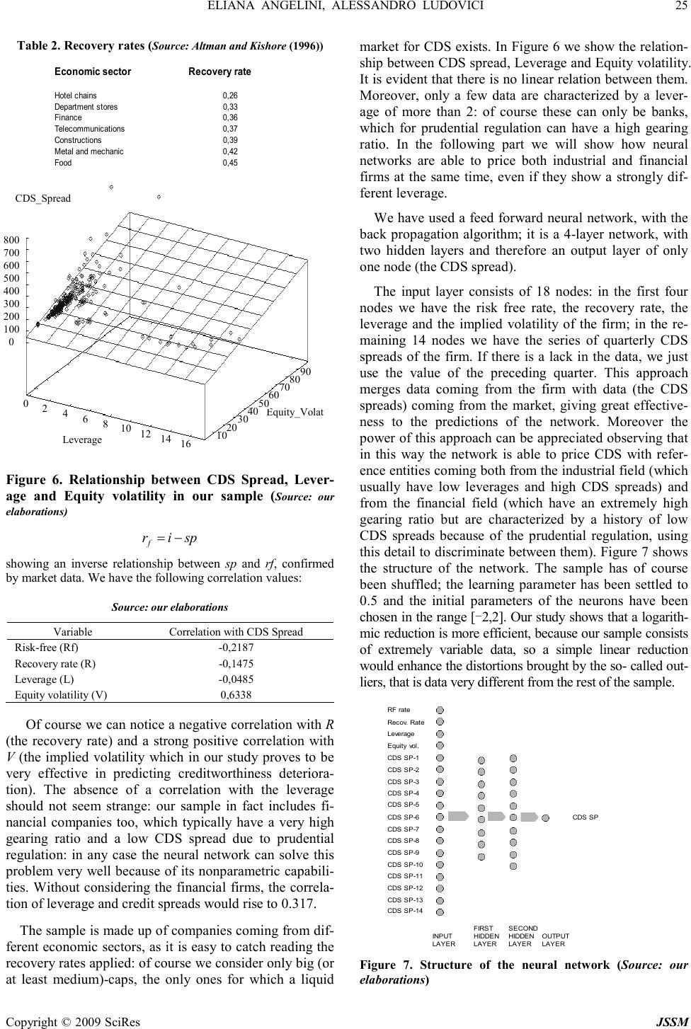

ELIANA ANGELINI, ALESSANDRO LUDOVICI 25
Table 2. Recovery rates ( Source: Altman and Kishore (1996))
Figure 6. Relationship between CDS Spread, Lever-
age and Equity volatility in our sample ( Source: our
elaborations)
spir
f
−=
showing an inverse relationship between sp and rf, confirmed
by market data. We have the following correlation values:
Source: our elaborations
Variable Correlation with CDS Spread
Risk-free (Rf) -0,2187
Recovery rate (R) -0,1475
Leverage (L) -0,0485
Equity volatility (V) 0,6338
Of course we can notice a negative correlation with R
(the recovery rate) and a strong positive correlation with
V (the implied volatility which in our study proves to be
very effective in predicting creditworthiness deteriora-
tion). The absence of a correlation with the leverage
should not seem strange: our sample in fact includes fi-
nancial companies too, which typically have a very high
gearing ratio and a low CDS spread due to prudential
regulation: in any case the neural network can solve this
problem very well because of its nonparametric capabili-
ties. Without considering the financial firms, the correla-
tion of leverage and credit spreads would rise to 0.317.
The sample is made up of companies coming from dif-
ferent economic sectors, as it is easy to catch reading the
recovery rates applied: of course we consider only big (or
at least medium)-caps, the only ones for which a liquid
market for CDS exists. In Figure 6 we show the relation-
ship between CDS spread, Leverage and Equity volatility.
It is evident that there is no linear relation between them.
Moreover, only a few data are characterized by a lever-
age of more than 2: of course these can only be banks,
which for prudential regulation can have a high gearing
ratio. In the following part we will show how neural
networks are able to price both industrial and financial
firms at the same time, even if they show a strongly dif-
ferent leverage.
We have used a feed forward neural network, with the
back propagation algorithm; it is a 4-layer network, with
two hidden layers and therefore an output layer of only
one node (the CDS spread).
The input layer consists of 18 nodes: in the first four
nodes we have the risk free rate, the recovery rate, the
leverage and the implied volatility of the firm; in the re-
maining 14 nodes we have the series of quarterly CDS
spreads of the firm. If there is a lack in the data, we just
use the value of the preceding quarter. This approach
merges data coming from the firm with data (the CDS
spreads) coming from the market, giving great effective-
ness to the predictions of the network. Moreover the
power of this approach can be appreciated observing that
in this way the network is able to price CDS with refer-
ence entities coming both from the industrial field (which
usually have low leverages and high CDS spreads) and
from the financial field (which have an extremely high
gearing ratio but are characterized by a history of low
CDS spreads because of the prudential regulation, using
this detail to discriminate between them). Figure 7 shows
the structure of the network. The sample has of course
been shuffled; the learning parameter has been settled to
0.5 and the initial parameters of the neurons have been
chosen in the range [-2,2]. Our study shows that a logarith-
mic reduction is more efficient, because our sample consists
of extremely variable data, so a simple linear reduction
would enhance the distortions brought by the so- called out-
liers, that is data very different from the rest of the sample.
Figure 7. Structure of the neural network (Source: our
elaborations)
Economic sectorRecovery rate
Hotel chains0,26
Department stores0,33
Finance 0,36
Telecommunications 0,37
Constructions 0,39
Metal and mechanic0,42
Food 0,45
CDS_Spread
Leverage
Equity_Volat
800
700
600
500
400
300
200
100
0
0
2
4
6
8
10
12
14
16
9
0
80
70
60
50
40
30
20
10
RF rate
Recov. Rate
Leverage
Equity vol.
CDS SP-1
CDS SP-2
CDS SP-3
CDS SP-4
CDS SP-5
CDS SP-6CDS SP
CDS SP-7
CDS SP-8
CDS SP-9
CDS SP-10
CDS SP-11
CDS SP-12
CDS SP-13
CDS SP-14
INPUT
LAYER
FIRST
HIDDEN
LAYER
SECOND
HIDDEN
LAYER OUTPUT LAYER

26 ELIANA ANGELINI, ALESSANDRO LUDOVICI
Figure 8. Typical correlogram of a CDS spread time serie
(Source: our elaborations)
In Figure 8 we show as an example the correlogram for
the CDS spread time series of The Boeing Company only,
for the sake of simplicity, but we obtained the same
structure for all the companies included in our sample: in
the first part we can see the correlation between each
value and a delayed value (the delay being expressed on
the x-axis); the second part shows the correlation be-
tween each value and p preceding values, with p on the
x-axis. It is therefore evident that the correlation between
values, even if decreasing, is strong, so the series is auto-
regressive; we can then express each value in terms of the
preceding ones. In this sense a CDS spread is more simi-
lar to an interest rate than to an equity price, so that it
shows a mean reversion process which tends to pull
spreads higher (lower) than some long-run average level
back to this value over time. Obviously we shall have a
negative (positive) drift. The sinusoidal cycle observable
in the correlogram explains this phenomenon: moreover,
it is a consequence of the strict relationship between CDS
spreads and risk-free interest rates already discussed [25].
Figure 9 showing in red the neural network predictions
and in yellow the real market data, confirms the effec-
tiveness of the neural network in predicting CDS spreads.
In Table 3 and 4 the values of R-squared and Rmse are
shown: as it is easy to observe, the results are highly co-
herent. We compare the results from or implementation
with another model: Creditgrades™. We must stress the
point that using traditional models such as Credit-
grades™ we would obtain predictions almost useless,
even excluding banks from the sample; neural networks
surely are a great pricing instrument in order to evaluate
credit spreads. The architecture of the neural network is
feed forward, trained for 17000 learning epochs using the
back propagation algorithm. Therefore it turns out obvi-
ous that neural networks are able to totally capture the
variability relative to the market dynamics of credit de-
rivatives: because of the fact that in literature there is no
unanimity on the determination of the form of the CDS
spread evaluation function, neural networks can therefore
be seen as effective instruments of elaboration able to
satisfy this lack from a statistical point of view.
Figure 10 shows a “delta” for a CDS contract: in fact
we find on the x-axis the leverage, and on the y-axis the
values calculated with the finite differences method, that is:
h
levSPhlevSP
h
)()(
lim
0
−
+
=∆
→
In a similar manner we can calculate for a CDS all the
“greek” letters typical of derivative contracts using the
outputs of the neural network with h-10
-6
. It is evident in
Figure 9. Market data (in yellow) and predictions of the
neural network (in red) ( Source: our elaborations)
Figure 10. Relationship between delta and leverage ( Source:
our elaborations )
Table 3. Approximation of the neural network ( Source: our
elaborations )
Error Value
R-squared 0,9082
Root mean squared error 14,3988
Table 4. Comparing statistical results (
Source: our elaborations )
NN Credit Grades Linear regression
Correlation 0,9636
-0,02 0,9309
Rmse 14,3988 >100 30,86
R-square 0,9086 >1 0,8566
010 20 3040 50 6070
0
25
50
75
100
125
150
175
200
225
250
275
300
325
350
Values and predictions
Values and predictions
0,010,1 0,18 0,27 0,36 0,45 0,54 0,63 0,720,8 0,88 0,97 1,06 1,15 1,24 1,33 1,421,5 1,58 1,67 1,76 1,85 1,94 2,03 2,122,2 2,28 2,37 2,46 2,55 2,64 2,73 2,822,9 2,98
-0,0125
-0,0100
-0,0075
-0,0050
-0,0025
0,0000
0,0025
0,0050
0,0075
0,0100
0,0125
0,0150
Delta(leverage)

ELIANA ANGELINI, ALESSANDRO LUDOVICI 27
Figure 10 shows a “delta” for a CDS contract: in fact
we find on the x-axis the leverage, and on the y-axis the
values calculated with the finite differences method, that is:
h
levSPhlevSP
h
)()(
lim
0
−
+
=∆
→
(20)
In a similar manner we can calculate for a CDS all the
“greek” letters typical of derivative contracts using the
outputs of the neural network with h-10
-6
. It is evident in
the diagram that for high leverages “delta” becomes
negative: in fact we must remember that highly leveraged
companies belong usually to the financial sector, so that
they are less risky because of the prudential regulation.
This effect is explained very well by the network, in fact
for low leverages (typical of the industrial field) we see a
direct relationship between leverage and CDS spreads. In
other words, the neural network is able to recognize the
risk of the activity carried out by the company using the
time series of its CDS spread: in the part of our study
covering the correlation, we obtained an average value
for each observation and the preceding one of 0.90, as it
is evident from the correlogram shown above. This cor-
relation, along with the part regarding the independent
variables, typical of the structural approach, explains the
major part of the variability of CDS spreads.
6. Conclusions and Future Work
In this paper we have discussed an innovative approach
to the study of CDS valuation, using neural networks.
Our analysis is based on modeling the underlying dy
Figure 11. Relationship between vega and equity volatility
(Source: our elaborations)
Figure 12. Relationship between gamma and leverage
(Source: our elaborations)
Figure 13. Relationship between omega and leverage
(Source: our elaborations)
namics of interest rates and firm characteristics and de-
riving the default probability based on these dynamics
(the structural approach).
The model that we propose is peculiar for the use of the
implied volatility of one-year options written on the shares
of the analyzed companies, instead of historical volatility.
Besides, the model differs from the structural approach for
the fact that it considers the 30-month historical series for
CDS spreads, including additional market variables. This
implementation allows to use a forward-looking model
and to capture the dynamic behavior of CDS spreads and
equity volatility. This approach merges data coming from
the firm with data (the CDS spreads) coming from the
market, giving great effectiveness to the predictions of
the neural network. Moreover, the power of this model
can be appreciated observing that in this way the network
is able to price CDS with reference entities coming both
from the industrial field (which usually have low lever-
ages and high CDS spreads) and from the financial field
(which have an extremely high gearing ratio but are
characterized by a history of low CDS spreads because of
the prudential regulation, using this detail to discriminate
between them).
We find that the neural network technique is useful for
analyzing the pricing of a credit default swap. Our model
produces a much lower forecasting error than those tradi-
tional models, such as Creditgrades
TM
, indicating a rela-
tively high precision in the neural network prediction. In
particular, in the last part, starting from the high correla-
tion observed between each CDS spread value and the
preceding one in the time series of each company, we
have trained a neural network based both on these time
series and on the structural details of the firms, that is
leverage, option-implied equity volatility and recovery
rates. Our results in terms of R-squared and Rmse are
highly coherent and are confirmed by the empirical data.
Our analysis presents the results that we have achieved
and shows that the neural network model offers an alter-
native to traditional methodologies to deal with compli-
cated issues related to CDS valuation.
Anyway, in this period, the CDS market is particularly
volatile. The impact on the economy of the deflating
0,54710
1418 22 26 30 3438 42 4650 5458 62 66 70 7478 8286 90 9498
-0,0200
-0,0180
-0,0160
-0,0140
-0,0120
-0,0100
-0,0080
-0,0060
-0,0040
-0,0020
0,0000
Vega(vol)
0,01 0,15 0,29 0,43 0,570,7 0,82 0,961,1 1,22 1,361,5 1,62 1,761,9 22,1 2,22 2,362,5 2,62 2,76
2,9 3
-0,0800
-0,0700
-0,0600
-0,0500
-0,0400
-0,0300
-0,0200
-0,0100
0,0000
0,0100
0,0200
Gamma (leverage)
0,01 0,14 0,27
0,40,50,60,70,80,91 1,11,21,31,41,51,61,71,81,92 2,12,22,32,42,52,62,72,82,93
-0,0900
-0,0800
-0,0700
-0,0600
-0,0500
-0,0400
-0,0300
-0,0200
-0,0100
0,0000
0,0100
0,0200
0,0300
Omega (leverage)

28 ELIANA ANGELINI, ALESSANDRO LUDOVICI
housing bubble, the credit crisis in general, have stoked
fear about increasing corporate defaults. This crisis is
about credit risk. A credit bubble has ballooned for years,
being enhanced by the existence of CDS. As credit origi-
nators can pass their risk to other agents, they have been
less careful about the quality of their loans. In that sense,
CDS have given an incentive for distributing more credit
to more risky borrowers. As banks and all financial insti-
tutions and companies have committed themselves in the
CDS market, they are now highly dependent on market
continuity and on its smooth functioning. The failure of a
major participant (bankruptcies of Bear Sterns, then those
of AIG and Lehman Brothers) can put at stake all the
others; the faith in the reliability of the market has been
deeply shaken by these events.
In any case, some aspects of the proposed evaluation
methodology require additional research: the possible next
step for the research community is to improve the models
in the case of catastrophic circumstances (the so-called
LFHI (low frequency-high impact) events); another in-
teresting case of study would regard the analysis of the
recent financial crisis when more reliable information
regarding financial companies will be available.
REFERENCES
[1] R. C. Merton, “On the pricing of corporate debt: The risk
structure of interest rate,” The Journal of Finance, 29 1974.
[2] S Henke, H. P. Burghof, and B. Rudolph, “Credit
securitization and credit derivatives: Financial instruments
and the credit risk management of middle market
com-mercial loan portfolios”, CFS Working paper Nr,
July 1998.
[3] A. Greenspan, “Economic flexibility,” Speech to HM
Treasury Enterprise Conference, London, UK, 2004.
[4] S. DAS, “Credit derivatives: Trading & Management of
Credit & Default Risk,” John Wiley & Sons, Chicago,
1998.
[5] J. M. Tavakoli, “Credit derivatives: A guide to instruments
and applications,” John Wiley & Sons, Chicago, 1998.
[6] G. R. Duffee and C. Zhou, “Credit derivatives in banking:
useful tools for managing risk?” Journal of Monetary
Economics, No. 48, 2001.
[7] R. Stultz, “Risk management and derivatives,” South-
Western Publishing, 2003.
[8] B. A. Minton, R. Stultz, and R.Williamson, “How much
do bank use credit derivatives to reduce risk?” Working
Papers, 2005.
[9] Bank for international settlement, “International convergence
of capital measurement and capital standards,” Basel Committee
on Banking Supervision, A Revised Framework, Update
November 2005.
[10] F. Dolcino, C. Giannini, and Rossi, E, “Reti neurali artificiali
per l’analisi e la previsione di serie finanziarie,” Collana
studi del Credito Italiano, 1998.
[11] D. Floreano and S. Nolfi, “Reti neurali: algoritmi di
apprendimento, ambiente di apprendimento, architettura,”
in Giornale Italiano di Psicologia, a. XX, pp. 15-50, febbraio
1993.
[12] M. Gori, “Introduzione alle reti neurali artificiali,” in Mondo
Digitale n. 4, AICA, settembre 2003.
[13] C. Wu and C. H.Yu, “Risk aversion and the yield of
corporate debt,” in Journal of Banking and Finance, No.
20, 1996.
[14] C. Wu, “A certainty equivalent approach to municipal
bond default risk estimation,” in Journal of Financial
Research, 1991.
[15] P. D. Mcnelis, “Neural networks in finance,” Elsevier
Academic Press, 2005.
[16] A. Beltratti, M. Serio, and P. Terna, “Neural networks for
economic and financial modelling,” International Thomson
Computer Press, 1996.
[17] S. Hykin, “Neural networks: A comprehensive foundation,”
Prentice Hall International, 1999.
[18] P. Werbos, “Backpropagation, past and future,” in Proceedings
of the IEEE International conference on neural networks,
IEEE press, 1988.
[19] F. Black and J. Cox, “Valuing corporate securities: Some
effects of bond indenture provisions,” Journal of Finance,
pp. 31, 1976.
[20] H. E. Lelan and K. B. Toft, “Optimal capital structure,
endogenous bankruptcy, and the term structure of credit
spreads,” The Journal of Finance, pp. 51, 1996.
[21] Collin dufresne and P. R. Goldstein, “Do credit spreads
reflect stationary leverage ratios,” Journal of Finance, pp.
52, 2001.
[22] R. A. Jarrow and S. M. Turnbull, “Pricing derivatives on
financial securities subject to credit risk,” The Journal of
Finance, pp. 50, 1995.
[23] R. Jarrow, D. Lando, and S. Turnbull, “A markov model
for the term structure of credit spreads,” Review of
Financial Studies, pp. 10, 1997.
[24] D. Duffie and K. J. Singleton, (1998), “Modelling term
structures of defaultable bonds,” Review of Financial
Studies, pp. 12, 1999.
[25] J. C. Hull, “Opzioni, futures e altri derivati,” Il Sole 24Ore
S. p. A., 2003.
(Edited by Vivian and Ann)