World Journal of Mechanics, 2012, 2, 311-324
doi:10.4236/wjm.2012.26037 Published Online December 2012 (http://www.SciRP.org/journal/wjm)
On the Modal and Non-Modal Model Reduction of
Metallic Structures with Variable Boundary Conditions
Wolfgang Witteveen
University of Applied Sciences Upper Austria, Wels, Austria
Received October 1, 2012; revised November 2, 2012; accepted November 12, 2012
ABSTRACT
Vibration mode based model reduction methods like component mode synthesis (CMS) will be compared to methods
coming from control engineering, namely moment matching (MM) and balanced truncation (BT). Conclusions based on
the theory together with a numerical demonstration will be presented. The key issues on which the paper is focused are
the reduction of metallic structures, the sensitivity of the reduced model to varying boundary conditions, full system
response, accurate statics and the possibility to determine “a priori” the number of needed modes (trial vectors). These
are important topics for the use of reduction methods in general and in particular for the implementation of FE models
in multi body system dynamics where model reduction is widely used. The intention of this paper is to give insight into
the methods nature and to clarify the strengths and limitations of the three methods. It turns out, that in the considered
framework CMS delivers the best results together with a clear strategy for an “a priori” selection of the modes (trial
vectors).
Keywords: Model Reduction; Vibration Modes; Component Mode Synthesis; Moment Matching; Balanced Truncation
1. Introduction
Model order reduction is a key issue when the dynamic
of finite element (FE) models is investigated. It is con-
cerned with the question whether a system with a large
number of degrees of freedom (DOF) n can be accurately
represented by a transformed system of the size m with m
<< n, see [1-3] for a general review and introduction on
this topic. During the last decades a lot of reduction
methods have been proposed. For linear elastic structures
with a moderate number of input degrees of freedom
(DOF), mode based reduction methods, like Component
mode synthesis (CMS) have been developed to very re-
liable standard tools. An overview of the family of CMS
methods is given by Craig in [4,5]. Another, more re-
cently published review has been done by de Clerk [6].
All CMS variants have in common, that at least a part of
the reduction base is formed by vibration modes. There-
fore this family of reduction methods will be denoted as
“mode” based within this work.
In the last few years a lot of effort has been made in
order to adapt model reduction methods for mechanical
structures which come originally from control engineer-
ing, namely moment matching (MM) and balanced trun-
cation (BT). In contrast to CMS where the trial vectors
have a physical meaning, the latter two methods are
based on mathematical considerations. Therefore MM
and BT are denoted as “non-modal” reduction methods.
In the following both approaches will be outlined as far
as it is necessary to understand the principal characteris-
tics and their consequences on the topic of this work.
More detailed introductions into MM which is also known
as “Krylov subspace method” can be found in [7-11] and
in case of BT the reader is referred to [12-15] for more
background information. In some newer publications
[16-19] the three methods have been compared to each
other and MM and BT have been pointed out as kind of
the “better method” with less error. In case of BT it has
been emphasized, that a “a priori” error bound in term of
displacements can be given, see among others [10,20,21].
This work deals with a critical qualitative comparison
of the three methods for industrial use of model reduction
for metallic structures with focus on the following im-
portant issues:
1) Sensitivity of the reduced system with respect to
varying boundary conditions;
2) Full system response;
3) Static and dynamic response;
4) Simple and clear strategy for an “a priori” selection
of the number of needed trial vectors.
1) Sensitivity of the reduced system with respect to
varying boundary condition: This is of particular impor-
tance for multi body dynamics where the implementation
of the component in the overall system is in general not

W. WITTEVEEN
312
known at the time when the reduction base is computed.
In this particular case an arbitrary interaction of the in-
put/output DOF with the surrounding rigid or flexible
bodies should be possible. The input/output DOF are those
on which external forces may be applied on the structure.
In other words, the response of the reduced system has to
be sufficient accurate independent of the stiffness or
mass which may be applied to the input/output DOF.
2) Full system response: MM and BT guarantee a de-
fined behavior between the input and output (I/O) of the
reduced system. The output vector holds a linear super-
position of the state vector and represents the quantity of
interest. This is of special interest in control engineering
but not sufficient in structural mechanics where accurate
stress recovery is an important requirement. For details
on stress recovery of reduced components, see [22-24].
Consequently, the response of the entire structure needs
to be considered because the place of the highest stress is
not known a priory and is not necessarily represented by
the I/O. For this reason this work is not focused on the
I/O behavior but on the full system response.
3) Static and dynamic response: In mechanics the static
response of a system is of special interest. It is not just a
theoretical issue as it may be in other disciplines. A static
portion in the overall system response leads to a mean
stress which influences the overall stress and therefore
the components lifetime. Neglecting the static in general
is not an option from a mechanical engineers point of
view.
4) Simple and clear strategy for an “a priori” selection
of the number of needed trial vectors: A key feature of a
reliable reduction method is a simple way to determine
the number of required modes in order to get an accurate
solution. No application engineer is interested in doing a
convergence analysis or a comparison with the full sys-
tem, as it is common in the academic society.
Note, that the applicability of the methods for huge FE
models is not issue of the current work, even it is still a
field of research, see [14] in case of BT. The focus is on
basic insights and qualitative differences.
There is already some comparative literature available,
see for example [25] and, as mentioned [16-19]. To the
best knowledge of the author the following points of this
paper have not been investigated and pointed out yet:
1) A comparison of the three methods with the focus
on the issues mentioned above, especially the varying
boundary conditions which are of significant importance
for the use of model reduction in multi body simulation.
2) The reliability of MM and BT in terms of statics.
3) The practical significance of the error bound of BT
when the boundary conditions of the input DOF in the
reduced system divers significant from the situation at
the time of trial vector generation.
4) The reliability of the methods when large parts of a
structure are not represented by the I/O. This is of par-
ticular interest when large models like car bodies or air-
crafts with few I/O locations will be reduced.
A preliminary und unfinished version of this work has
been published at the SEM IMAC Conference in Jack-
sonville, FL, US [26].
The paper is organized as follows: In a first section
general issues connected to model reduction will be dis-
cussed as well as issues arising from the prior mentioned
topics. In the subsequent section all three approaches will
be briefly outlined as far as it is necessary to see the
qualitative differences. At the end of this chapter the
most important conclusions already can be drawn based
on the given equations. In the following a simple beam
example is used to demonstrate the expected advantages
and disadvantages of each method which leads to a clear
conclusion and recommendation. Finally some publica-
tions will be briefly discussed.
2. General Issues on Model Reduction of
Metallic Structures
The FE method leads to an equation of motion in the
form of
1
1



Mx KxBu
yCx (1)
where the (n × n) matrixes M and K are the mass and
stiffness matrix, the (n × 1) vector x contains the bodies
DOF, the (u × 1) vector u holds the time history of the
applied loads, the (n × u) matrix B1 maps the loads to the
corresponding degrees of freedom, the (y × 1) vector y
holds the output of interest and C1 maps the state vari-
ables to the output. In the following a symmetric system
is considered with M = MT and K = KT. In next subsec-
tion it will be discussed why no viscous damping is con-
sidered for the reduction process.
The corresponding reduced system can be given as
1
1
1111
,,,
,
TT
T


 




 
MzKzB u
yCz
xVzMWMV KWKV
B=W BC=CV
(2)
with the (m × 1) vector z and the (n × m) matrixes V and
W. Model order reduction deals with the question of de-
termining the matrixes V and W, so that the reduced sys-
tem captures somehow the important characteristics of
the unreduced system.
For a better readability of this work it is remembered
that (1) can be transformed into a first order system in the
form of

W. WITTEVEEN
313

1
1
,,
,
TTT








 

 

 
00
00
00


EqAq Bu
yCq
qxxB CC
B
II
EA
MK
(3)
In [15] a little modification of (3) is suggested, so that
symmetric system matrixes E and A are obtained:
,



 

 

 
00
00

E
qAqBu
yCq
K
K
EA
MK
(4)
The latter modification has some important implica-
tions which will be reported in subsection 2.2. The ac-
cording reduced system is
,,
,
TT
T


 

 


 

 
EqAq Bu
yCq
qVqEWEV AWAV
BWBCCV
(5)
with the (2n × m) reduction matrixes V and W.
2.1. Absence of the Viscose Damping Matrix
The damping matrix is not considered in Equation (1)
because of the nature of the two most frequently involved
dissipation mechanisms, namely material damping and
joint damping (micro slip). Both of them are energy dis-
sipation mechanisms which cannot be properly modeled
by pure viscous damping. Material damping of metallic
structures will be overestimated in case of high fre-
quency if it is modeled with a viscous damping matrix,
see [27-29] for an experimental verification with alumi-
num. The reason why material damping is commonly
modeled with a velocity proportional approach is more
its simplicity than its accuracy. Furthermore it is mention
worth that material damping of metallic structures is that
low so that it is normally dominated by other damping
mechanisms like joint damping or by external applied
damping like rubber bearings, lubrication bearings or the
like. Joint damping (micro slip) is frequently independent
and cannot be modeled by a viscous damping at all, see
exemplarily [30]. Consequently, a viscous damping is
always an inaccurate approximation for metallic struc-
tures and it does not matter if it is introduced in the full
system or in the reduced system. When the damping ma-
trix is regarded in the reduction process, it will influence
the final comparison between the reduced and the full
model. This doesn’t make sense because something physi-
cally not meaningful is introduced and may affect an
objective evaluation. Note, that the latter considerations
may not be valid for structures with a large amount of
rubber, plastic or other visco-elastic materials.
2.2. Stability and Symmetry of the Reduced
System
If the reduced model (2) is used for time integration it is
of significant importance, that no instability will be in-
troduced due to the model reduction. In this particular
case, when no damping is regarded the eigenvalues of the
reduced model are required to be real, such as they are in
the original system. The symmetry of a mechanical sys-
tem is a fundamental characteristic which should be pre-
served during the reduction process.
Both is obtained in case of a so called “symmetric or
single sided projection” which requires an identical re-
duction and test space matrix

WV (6)
In case of a symmetric system (4) and when the input
DOF are the same as the output DOF

11
TCB it has
been demonstrated in [7] and [15], that MM and BT
leads to a symmetric projection (6).
Note, that the latter, more mathematical considerations
do have a mechanical pendant. In case of a coordinate
transformation it is common in mechanics to apply the
principle of virtual work, which requires, that the work of
all forces due to a virtual displacement has to vanish.
This can be written as


1
T


0

xMxKxBu (7)
where δ indicates a virtual displacement of the state vec-
tor. If the reduction law x = Vz is used for the state vector
as well as for the virtual displacement the reduced system
(2) is obtained with W = V. For the latter reasons we re-
strict ourselves to such systems where 11
TCB.
3. Brief Review on Component Mode
Synthesis, Moment Matching and
Balanced Truncation
For the sake of simplicity and readability an invertible
stiffness and mass matrix will be assumed further one.
The presence of rigid body modes doesn’t have an effect
on the conclusions which will be drawn. As mentioned
before, the theory given next is by far not exhaustive but
should give at least as much insight, that the finally
drawn conclusions are understandable.
3.1. Component Mode Synthesis, See [4-6]
A CMS based reduction is typically directly applied to
the second order system (1). Commonly, the reduction
matrix is of the form

W. WITTEVEEN
314


SD
VVV
(8)
where the trial vectors in the (n × p) matrix VD are vibra-
tion modes which capture the systems dynamics. These
modes are obtained by a proper eigenvalue problem
which delivers the modes eigenfrequencies. For the re-
duction process just those p modes (p << n) are regarded,
having an eigenfrequency smaller as a defined limit,
which typically a factor of 1.5 - 2 higher as the highest
relevant frequency content of all involved forces.
In order to improve the convergence, some static trial
vectors are added to the vibration modes. These trial
vectors are obtained by loads on the input/output DOF
and collected in the columns of the (n × s) matrix VS.
During the last decades a lot of methods for the com-
putation of V according to (8) have been suggested. An
overview is given by Craig in [5]. In the latter publica-
tion it has been shown, that the different approaches span
a similar space. For this publication the most frequently
used method has been chosen to represent the family of
“mode based” reduction methods, namely the fixed
boundary CMS introduced by Craig (and Bampton) [31].
According to Craig’s method the vector of nodal DOF
of the FE model is subdivided into
TTT
B
I

 xxx (9)
where the (b × 1) vector xB represents the “boundary”
DOF and the


1nb vector xI holds the remaining‚
inner DOF. The boundary DOF is those DOF on which
external forces may be applied. In this work these DOF
are mostly denoted as input/output DOF. In terms of (1),
the input matrix B1 contains non zero entries at these
DOF. According to the subdivision (9), an eigenvalue
problem in the form of
2
,,,IIiII Di




0KMv
(10)
can be used for the computation of the vibration modes.
The
 
nb nb matrixes KI,I and MI,I denote the
portion of K and M matching the definition of (9). The
obtained modes vD,i are named as ‚Fixed Boundary Nor-
mal Modes’ and can be given as
,1 ,2,
D
D
DDp



0000

Vvv v (11)
with an user defined eigenfrequency limit ω* so that
p



 (12)
As mentioned before, the latter limit is usually con-
nected to the highest relevant frequency content of the
excitation. Die Matrix VS is obtained according to a
Guyan [32] reduction
1
,,
S
I
IIB





I
VKK (13)
with the (b × b) identity matrix I. Obviously, each boun-
dary DOF introduces a trial vector in VS.
It is known that the use of such static displacement
fields significantly improve the convergence of the solu-
tion in case of imposed boundary conditions which are
different to the one at the time of mode generation, see
reference [24]. Therefore it is to expect, that CMS should
deliver good results independently of the applied bound-
ary conditions. This is an important feature for accurate
stress recovery as well, see [24].
Unfortunately no “a priori” error bound in terms of
displacement is known yet. However, the procedure en-
sures exact statics and the presence of all modes of inter-
est within a well defined frequency range.
3.2. Moment Matching, See [7-11]
With the Laplace transformation the transfer function of
the system (4) can be given as
 
1
ss 
H
CEA B
(14)
where s holds the complex Laplace variable. An ap-
proximation of (14) with a Power Series around s0 gives
 
0
0
0
j
s
j
j
s
ss




HT (15)
with the so called j-th moment.




011
00
j
s
jss

 TCEAEEAB (16)
see [7]. If W and V are chosen in such a way that the
spanned space is equal to



110
11
110
11
m
m
vv vvv
m
m
WW WWW

















Vv vv
PR PRR
Ww ww
P
RPRR
(17)
with




1
0
1
0
0
0
v
v
TT
W
TT
v
s
s
s
s








REAB
PEAE
REAC
PEAE
(18)
it can be shown, that the first 2 m moments of the re-
duced system around s0 are equal to those in the full sys-
tem.
00 1,, 2
ss
jj jm

TT (19)
Note, that a direct implementation of (17) for the con-
struction of W and V is numerically disadvantageous.
The literature offers better choices, see exemplarily [11].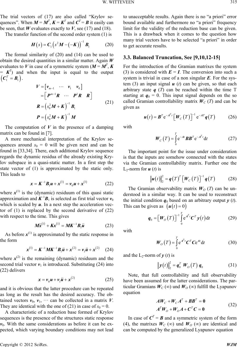

W. WITTEVEEN
315
The trial vectors of (17) are also called “Krylov se-
quences”. When M = MT, K = KT and CT = B it easily can
be seen, that W evaluates exactly to V, see (17) and (18).
The transfer function of the second order system (1) is
 

1
2
11
ss  
H
CM KB (20)
The formal similarity of (20) and (14) can be used to
obtain the desired quantities in a similar matter. Again W
evaluates to V in case of a symmetric system (M = MT, K
= KT) and when the input is equal to the output

11
TCB.




110
11
1
2
01
1
2
0
m
m
s
s











Vv vv
PR PRR
RMKB
PMKM
(21)
The computation of V in the presence of a damping
matrix can be found in [7].
A more mechanical interpretation of the Krylov se-
quences around s0 = 0 will be given next and can be
found in [33,34]. There, each additional Krylov sequence
regards the dynamic residua of the already existing Kry-
lov subspace in a quasi-static matter. In a first step the
state vector of (1) is approximated by the static only.
This leads to
 
11
1
10

xKBux vux (22)
where x(1) is the (dynamic) residuum of this quasi static
approximation and K–1B1 is selected as first trial vector v0
which is scaled by u. In a next step the acceleration vec-
tor of (1) is replaced by the second derivative of (22)
with respect to the time. This gives
 
11 1
1


 
MxKxMKBu (23)
As before x(1) is approximated by the static response in
the form
 
122
11
11


 
xKMKBuxvux (24)
where x(2) is the remaining (dynamic) residuum and the
second trial vector v1 is introduced. Substituting (24) into
(22) delivers

2
01


xvuvux (25)
and it is obvious that the latter procedure can be repeated
as long as the result has the desired accuracy. The ob-
tained vectors v0, v1, ··· can be collected in a matrix V.
They are identical with the one of (21) in case of s0 = 0.
A characteristic of a reduction base formed of Krylov
sequences is the presence of the structures static response
v0. With the same considerations as before it can be ex-
pected, which varying boundary conditions may not lead
to unacceptable results. Again there is no “a priori” error
bound available and furthermore no “a priori” frequency
limit for the validity of the reduction base can be given.
This is a drawback when it comes to the question how
many trial vectors have to be selected “a priori” in order
to get accurate results.
3.3. Balanced Truncation, See [9,10,12-15]
For the introduction of the Gramian matrixes the system
(3) is considered with E = I. The conversion into such a
system is trivial in case of a non singular E. For the sys-
tem (3) an input signal u (t) can be given, so that each
arbitrary state q (T) can be reached within the time T
starting at q0 = 0. This input signal depends on the so
called Gramian controllability matrix WC (T) and can be
given as
 
1
ee
T
Tt T
C
tTT




AA
uB Wq (26)
with

0
eed
T
T
tT t
CTt

AA WBB
(27)
The important point for the issue under consideration
is that the inputs are somehow connected with the states
via the Gramian controllability matrix. Further one the
L2-norm for u (t) is
 
21
2
T
C
tT TT



uqWq (28)
The Gramian observability matrix WO (T) can be un-
derstood in a similar way. It can be used to reconstruct
the initial condition q0 based on an arbitrary output y (t).
This can be given as




0t

u
 
1
0
0
ed
T
T
tT
OTtt


 A
qWCy (29)
with

T
0
eed
T
tT t
OTtAA
WCC
(30)
and the L2-norm of y (t) is
 
2
00
2
T
O
tTyqWq (31)
Note, that full controllability and full observability
have been assumed for the latter considerations. The par-
ticular Gramians WC (∞) und WO (∞) fulfill the Lyapunov
equation
TT
CC
TT
OO




0
0
AWWABB
AWWAC C
(32)
In case of CT = B and a symmetric system of the form
(4), the matrixes WC (∞) und WO (∞) are identical and
can be computed by the generalized Lyapunov equation

W. WITTEVEEN
316
TT
T
CC
 
 

 0ΕWA AWΕBB (33)
see [15]. At this point it is important to note, that system
(4) und its Gramians are not unique. With each non sin-
gular (2 n × 2 n) matrix T* a transformation in the form
of

 qTq (34)
can be performed which leads to an equivalent but dif-
ferent system. A system is called “balanced” when the
Gramians are diagonal and WC = WO. The corresponding
transformation is unique and the transformation matrix
will be denoted as T. For the balanced system, Equation
(28) evaluates to
  
 
1
2
2
2
2
1
1
1
1
T
n
n
ii
ii
tTT
qT qT
















uq q
(35)
with σ1 > σ2 > ··· > σ2n. Equation (35) gives insight how
the energy of the input signal is distributed among the
states which correspond to the vectors of the transforma-
tion matrix T. A small σj leads to a large 1
j

 and that
means that the vector j needs a lot of energy from the
input signal to be controlled. Equation (31) can be writ-
ten as

1
2
00
2
2
2
0, 0,
1
T
n
n
ii i
i
t
qq










 

yq q
(36)
and it gives insight how the energy of the output signal
depends from the. A large value of σj means, that the
energy of the output signal is strongly influenced by this
particular state.
The idea of BT is, to use just these states which need
low energy to be controlled from the input and which
give a lot of energy to the output. Note, that the values of
σj decrease very quickly for common mechanical struc-
tures so that just a view columns of the transformation
matrix need to be considered as trial vectors for model
reduction. A special feature of this approach is an “a pri-
ori” error bound in the form of
22
δBT u

yy (37)
with
2
1
2
n
B
Tj
jm



 (38)
and m as the number of the last considered trial vector,
see exemplarily [10,20,21].
Note, that the upper error bound (38) is just valid for a
balanced realization of a first order LTI system in the
form of (4) or (3) and does not hold when BT is direct
applied to second order systems (1). A direct application
of BT on second order systems is somehow different.
Instead of single controllability and observability Gramian
matrixes there are Gramians for the positions and veloci-
ties. The interested reader is referred to [6,13] for a de-
tailed discussion and more literature quotations. In [9,16]
a modified error bound has been developed for such sys-
tems in case of frequency weighted Gramians. For more
literature on actual implementations of BT for first order
LTI systems and second order systems see [9,10,12-15].
In [35] the use of MM together with BT has been sug-
gested. MM is used there in order to transform a huge
system into one of moderate size. In a subsequent step
BT has been applied in order to transform the moderate
system into one of small size.
The Gramians obtained by the Lyaponov equations
consider all frequencies but a direct solution can be very
expensive for large systems. It is possible to compute or
approximate the Gramians for a frequency range of in-
terest, see [9] or [20]. A low rank approximation of the
solution of the Lyaponov equation can be found in [36].
One approach for the reduction of second order sys-
tems with an approximated position controllability Gramian
is reported in [9] and given next. It delivers valuable
qualitative insight into the nature of BT, especially in the
framework of un- or lightly damped structures. Similar
considerations can be found in [20] for arbitrary first
order LTI systems.
In a first step a series of frequency response computa-
tions of (1) for k frequencies in the form of


2
1 Limit
01
iii ik


 MKX B (39)
have to be carried out. The resulting (n × u) deformation
matrixes Xi are collected in the


nku matrix


2ik

X
XX X. (40)
In a subsequent step the matrix X is decomposed in its
Proper Orthogonal Modes (POM) by using Proper Or-
thogonal Decomposition (POD) which is also known as
Karhunen-Leove decomposition. The interested readers
are referred to [37,38] for a short review on the POD
itself and on the available literature. In [39] a detailed
outline of the theoretical background can be found. Due
to the definition of POD the first m POM v1 ··· vm can be
characterized as

W. WITTEVEEN
317






1
2
2
11 1
,,
2
2
1
max
..
n
m
TT
kxu
TT
mm
kxu
T
ji ij
st 

 









uu
xvx v
xvx v
vv
(41)
where δij denotes Kroneckers delta. The vectors v1 ··· vm
can be interpreted as those which span “most” of the
space of X in a Euclidean sense. Note that the POM are
the eigenvectors of XXT and the magnitude of the ac-
cording eigenvalues correlate with the importance of a
POM, analog the entries σi of (35) and (36). For a lot of
mechanical systems these eigenvalues decrease rapidly
so that m << n. Finally the vectors v1 ··· vm will be used
for the reduction matrix V. As observed in [9] the matrix
XXT is an approximation of the position controllability
Gramian which is the link of this approach to BT.
In [40] it has been demonstrated, that the POM of an
undamped system with a mass matrix proportional to the
identity matrix are identical with the free vibration
modes. This observation can be generalized to systems
where M and K fulfill the criteria given in [41]. The latter
publication focuses on necessary and sufficient condi-
tions so that the vibration modes are orthogonal with
respect to the mass and stiffness matrix and to them-
selves. Note, that the vibration modes orthogonality with
respect to themselves is not true in general.
For the following considerations it is assumed that the
number of frequency samples k off (39) is high enough
so that each reachable vibration mode will be excited
nearby its eigenfrequency. Therefore each excited eigen-
frequency will lead to huge contributions in X. Now it
can be concluded that the space spanned by X is domi-
nated by these (linear independed) vibration modes. The
later considerations and (41) require that the first and
most important POM approximate the space spanned by
the dominating vibration modes.
The fact that the conservative system may have infi-
nite response, implies that the “a priori” error estimation
(37) is just valid in presence of a viscous damping which
is not realistic in the framework of metallic structures,
see the remarks in chapter 2.1. This is the first observa-
tion why the “error controlled model reduction” is more a
theoretical statement than a practical one, when applied
to the reduction of metallic structures.
The static response of the structure is undetermined
because in general it cannot be ensured that it can be ap-
proximated by a space spanned by the vibration modes.
Especially when the static response in a dynamical stiff
direction is needed, the displacement error may be small
but the error in terms of stress is not predictable which is
demonstrated in the numerical example below. Note that
in a dynamic response computation the exact representa-
tion of a static portion is very important because it leads
to mean stress which is a significant parameter for fa-
tigue lifetime prediction.
In terms of dynamics, it is known that static deflection
shapes, which help to fulfill arbitrary boundary condi-
tions, do accelerate the convergence of a mode base [24].
Therefore it is to expect, that a balanced reduced system
does not deliver accurate results in case of mounted or
mistuned I/O DOF. The observation that the absence of
static displacement fields may lead to considerable errors
can be found in [42] as well. This publication deals with
the application of POD to linear dynamic systems. The
relation to BT is not mentioned there. However, a sug-
gestion is given to improve the reduction base by a static
correction.
Finally it is important to emphasize the difference be-
tween the eigenfrequencies of (10) and the singular val-
ues (SV) σi of (35) and (36). An eigenfrequency has a
physical meaning and denotes a pole in the system char-
acterized by M and K. The SV describes the importance
of a trial vector in terms of a Euclidean distance or an
energy transfer from the input to the output. This differ-
ence leads to two interesting facts:
 A certain mode will not be detected by BT when the
locations of the input/output DOF are at this modes
vibration node.
 The sequence of the POM is not directly connected
with the eigenfrequencies of the structure but with the
location of the input/output DOF. That means that
there is no direct correlation between the number of
trial vectors and spanned frequency range.
3.4. Short Remark on the Number of Input/
Output DOF
As it can be seen in the theory outlined before, the num-
ber of I/O DOF is kind of a bottle neck. Too many of
such DOF would lead to many columns in the reduction
matrixes and therefore to an undesired size of the re-
duced model. Model reduction for systems with many
input/output DOF is still an active field of research and
the interested reader is referred to [43-45] for some dif-
ferent approaches to overcome that problem.
3.5. Summary and Conclusions Based on the
Nature of the Three Approaches
1) Using CMS in a proper way leads to a reduced sys-
tem which is exact in terms of static and sufficient for a
defined range for frequency. It is to expect that the static
mode shapes will guarantee satisfying results even if the
I/O DOF is different mounted as at the time of mode gen-
eration.
2) MM leads to an exact static behavior whereas the
dynamics is not clearly predictable because no frequency
range of validity can be given for a certain number of

W. WITTEVEEN
318
trial vectors.
3) It is to expect, that the strength of MM and BT is
the representation of the I/O characteristic of the full
system in the reduced space. The error is a minimum and
even predictable in case of BT when no statics is of sig-
nificance.
4) For BT it can be expected that the static response is
in general not accurate. The dynamic response is not ac-
curate for a reduced system with different boundary con-
ditions as they have been at the time of mode generation.
4. Numerical Example (Cantilever Beam)
In the latter section some conclusions have been drawn
just by considering the characteristics of the reduction
methods. A generic beam example will be investigated
for a practical demonstration of the former insights.
As mentioned before a non floating structure (invert-
ible stiffness matrix) is considered in order to keep the
formalism as simple as possible without losing generality.
There is no single conclusion which would not hold in
case of a floating structure.
The beam seems a bit artificial, especially the over-
hanging sub beam. The intention was the presence of a
significant part which is not covered by the input/output
DOF. This is of practical relevance for the model reduc-
tion of large structures like car bodies or aircrafts. In
such cases it cannot be garneted in general, that the criti-
cal regions which are not known “a priori” are well rep-
resented by the I/O.
4.1. FE Model and Investigated
Figure 1 contains a visual representation of the FE model
of the beam structure. The beam has been modeled using
the CBEAM1 elements of the FE code MSC.NASTRAN
[46]. The square of the bottom section is of 100 mm by
Figure 1. Solid and wireframe representation of the FE
model under consideration.
10 mm and the one of the overhanging beam is 100 mm
by 5 mm, the Young’s modulus is of 210,000 N/mm2, the
shear modulus is of 80,000 N/mm2 and the density is of
7800 kg/m3. The structure is mounted at the grid point
where the coordinate system is located and 6 input/out-
put DOF are located at the free end of the beam which is
denoted as A and marked in Figure 1 by a circle. One
additional input/output DOF in z direction is located at
the center of the beam which is denoted as B and marked
in Figure 1 as well. Note, that the sub beam which has
its main extension in x direction will be denoted as “bot-
tom section” further one.
The mass and stiffness matrixes have been assembled
by MSC.NASTRAN [46] and exported to an ASCII File.
The content of this ASCII File has been imported to
Scilab [47] which was used for all subsequent computa-
tions.
For the evaluation of the reduction methods, the re-
duced model will be compared to the full model with
respect to statics and dynamics. In order to evaluate the
statics, simply the static deflection shapes due to certain
loads is computed in the full and in the reduced system.
The dynamics is evaluated by a comparison of the ei-
genvectors and eigenvalues of the full and the reduced
system.
Three different variants will be investigated. Note, that
the reduction base is equal for all of them. The changes
are applied at the reduced model only.
Variant 1: No additional boundary conditions are ap-
plied in the reduced system. Consequently the system is
equal to the one at the time of mode (or trial vector) gen-
eration.
Variant 2: All 6 DOF of point A will be fixed to ground.
Variant 3: All translational and rotational DOF of point
A will be fixed to ground except the translation in x di-
rection. This is similar to a “sliding” joint. An additional
mass is mounted at point A.
4.2. Error Measures
The static results will be compared by plotting the bend-
ing lines in the direction of interest. The dynamics of the
reduced system will be evaluated by means of the rela-
tive error of the frequencies and the MAC value of the
normalized mode shapes. The error in frequency of mode
number i is measured as
ii
i
i
f
f
f




(42)
and the MAC value of the corresponding mode shapes is
defined as


2
T
ii
iTT
ii ii





 (43)

W. WITTEVEEN
319
where βi has a value between 0 and 1 and 1 means full
identity, see [48]. Figure 2 helps to get an impression
what βi = 0.95 means in terms of displacements. For that
reason, a value of βi < 0.95 will be denoted as inaccurate
further one.
4.3. Model Reduction
4.3.1. Moment Matching
As it can be seen in (21), moment matching leads to
blocks which are added to the reduction matrix. Due to
the 7 selected I/O DOF the number of trial vectors in the
reduction matrix is an even multiple of 7. For this study a
total number of 14 trial vectors have been selected. The
trial vectors have been computed along the algorithm
cited in [11].
4.3.2. CMS
The Craig-Bampton approach [31] requires 7 static dis-
placement vectors and a number of vibration modes which
can be estimated by the frequency content of the excita-
tion. As mentioned before, the final size of the entire
reduction matrix is given by the MM approach which
leads to 7 fixed interface vibration modes which are
added to the CMS reduction base. The highest considered
frequency is about 331 Hz. Therefore, as an “a priori”
estimation, the eigenvalue and eigenvectors should be
accurate up to approx. 200 Hz.
4.3.3. BT
The trial vectors based on balanced truncation have been
computed along the SBPOR algorithm of [15]. This al-
gorithm requires the presence of viscous damping. There-
fore a damping matrix D = 1.0e–4K has been defined in
order to obtain the trial vectors.
In Chapter 3.3, it has been assumed, that in case of full
controllability the space spanned by balanced truncation
is somehow similar to one spanned by the systems vibra-
tion modes. For a numerical confirmation of that as-
sumption the first three vibration modes of the structure
have been put into a matrix. A singular value decomposi-
tion of this matrix delivers the Hankel singular values
(HSV) 2.6, 2.2 and 1.4. In a next step the first three trial
vectors obtained by the SBPOR algorithm have been
added to the matrix which contains the three vibration
modes. The HSV of this matrix are 2.7, 2.4, 1.7, 0.006,
0.0001 and 0.0000002. The sudden decrease of HSV
reveals that this 6 dimensional space is dominated by
three dimensions. Consequently, both groups of modes
Figure 2. Two mode shapes with βi = 0.95.
(or trial vectors) span a similar space.
4.4. Variant 1: Reduced System with the Same
Boundary Conditions as at the Time of Mode
Generation
4.4.1. Stati c Response
Two different static load cases will be investigated.
Load Case 1 (LC 1): Two forces in z direction have
been applied. One about 50 N at point B and another one
about –15 N at point A.
Load Case 2 (LC 2): A single force in x direction
about 1000 N has been applied at point A.
The resulting deflection in z direction of the bottom
section due to LC 1 can be seen in Figure 3. As it was
expected the CMS and MM reduced model deliver accu-
rate results while BT does not.
The resulting deflection in x direction of the bottom
section due to LC 2 can be seen in Figure 4. This is a
very interesting result. It underlines the advantage of
static displacement shapes as trial vectors. While the
CMS and MM results are exact the BT result is highly
inaccurate. This is, because no trial vector with a domi-
nate displacement in x direction is part of the reduction
base. The reason for this is the displacement oriented
reduction procedure where directions with high dynamic
stiffness are considered to be less important, see (41).
The latter observation has important consequences for
the dynamoics as well. If an arbitrary dynamic response
contains a quasi static portion of the latter deflection in x
direction, the resulting stress state will be inaccurate even
if the displacement error may be small. The missing
mean stress would lead to bad fatigue lifetime prediction
as well.
4.4.2. Dynamics
Figure 5 contains a summary of the eigenfrequency errors
and the correlations of the according mode shapes, re-
spectively. It can be seen that up to 200 Hz, which is the
“a-priori” assumed range of validity for CMS, all meth-
Figure 3. z-deflection of bottom section due to LC 1.
Figure 4. x-deflection of bottom section due to LC 2.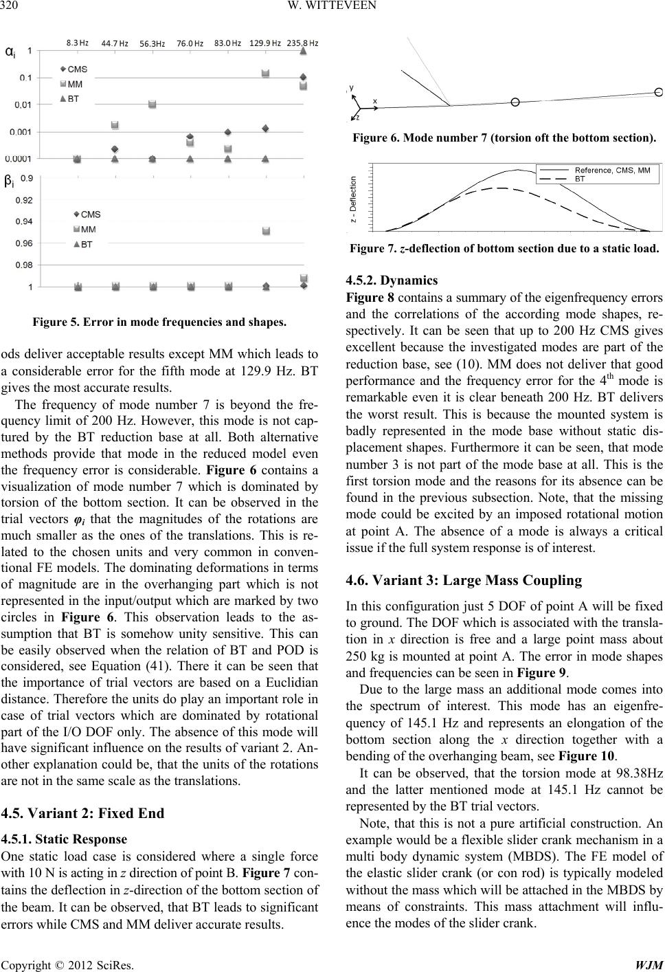

W. WITTEVEEN
320
Figure 5. Error in mode frequencies and shape s.
ods deliver acceptable results except MM which leads to
a considerable error for the fifth mode at 129.9 Hz. BT
gives the most accurate results.
The frequency of mode number 7 is beyond the fre-
quency limit of 200 Hz. However, this mode is not cap-
tured by the BT reduction base at all. Both alternative
methods provide that mode in the reduced model even
the frequency error is considerable. Figure 6 contains a
visualization of mode number 7 which is dominated by
torsion of the bottom section. It can be observed in the
trial vectors φi that the magnitudes of the rotations are
much smaller as the ones of the translations. This is re-
lated to the chosen units and very common in conven-
tional FE models. The dominating deformations in terms
of magnitude are in the overhanging part which is not
represented in the input/output which are marked by two
circles in Figure 6. This observation leads to the as-
sumption that BT is somehow unity sensitive. This can
be easily observed when the relation of BT and POD is
considered, see Equation (41). There it can be seen that
the importance of trial vectors are based on a Euclidian
distance. Therefore the units do play an important role in
case of trial vectors which are dominated by rotational
part of the I/O DOF only. The absence of this mode will
have significant influence on the results of variant 2. An-
other explanation could be, that the units of the rotations
are not in the same scale as the translations.
4.5. Variant 2: Fixed End
4.5.1. Stati c Response
One static load case is considered where a single force
with 10 N is acting in z direction of point B. Figure 7 con-
tains the deflection in z-direction of the bottom section of
the beam. It can be observed, that BT leads to significant
errors while CMS and MM deliver accurate results.
Figure 6. Mode number 7 (torsion oft the bottom section).
Figure 7. z-deflection of bottom section due to a static load.
4.5.2. Dynamics
Figure 8 contains a summary of the eigenfrequency errors
and the correlations of the according mode shapes, re-
spectively. It can be seen that up to 200 Hz CMS gives
excellent because the investigated modes are part of the
reduction base, see (10). MM does not deliver that good
performance and the frequency error for the 4th mode is
remarkable even it is clear beneath 200 Hz. BT delivers
the worst result. This is because the mounted system is
badly represented in the mode base without static dis-
placement shapes. Furthermore it can be seen, that mode
number 3 is not part of the mode base at all. This is the
first torsion mode and the reasons for its absence can be
found in the previous subsection. Note, that the missing
mode could be excited by an imposed rotational motion
at point A. The absence of a mode is always a critical
issue if the full system response is of interest.
4.6. Variant 3: Large Mass Coupling
In this configuration just 5 DOF of point A will be fixed
to ground. The DOF which is associated with the transla-
tion in x direction is free and a large point mass about
250 kg is mounted at point A. The error in mode shapes
and frequencies can be seen in Figure 9.
Due to the large mass an additional mode comes into
the spectrum of interest. This mode has an eigenfre-
quency of 145.1 Hz and represents an elongation of the
bottom section along the x direction together with a
bending of the overhanging beam, see Figure 10.
It can be observed, that the torsion mode at 98.38Hz
and the latter mentioned mode at 145.1 Hz cannot be
represented by the BT trial vectors.
Note, that this is not a pure artificial construction. An
example would be a flexible slider crank mechanism in a
multi body dynamic system (MBDS). The FE model of
the elastic slider crank (or con rod) is typically modeled
without the mass which will be attached in the MBDS by
means of constraints. This mass attachment will influ-
ence the modes of the slider crank.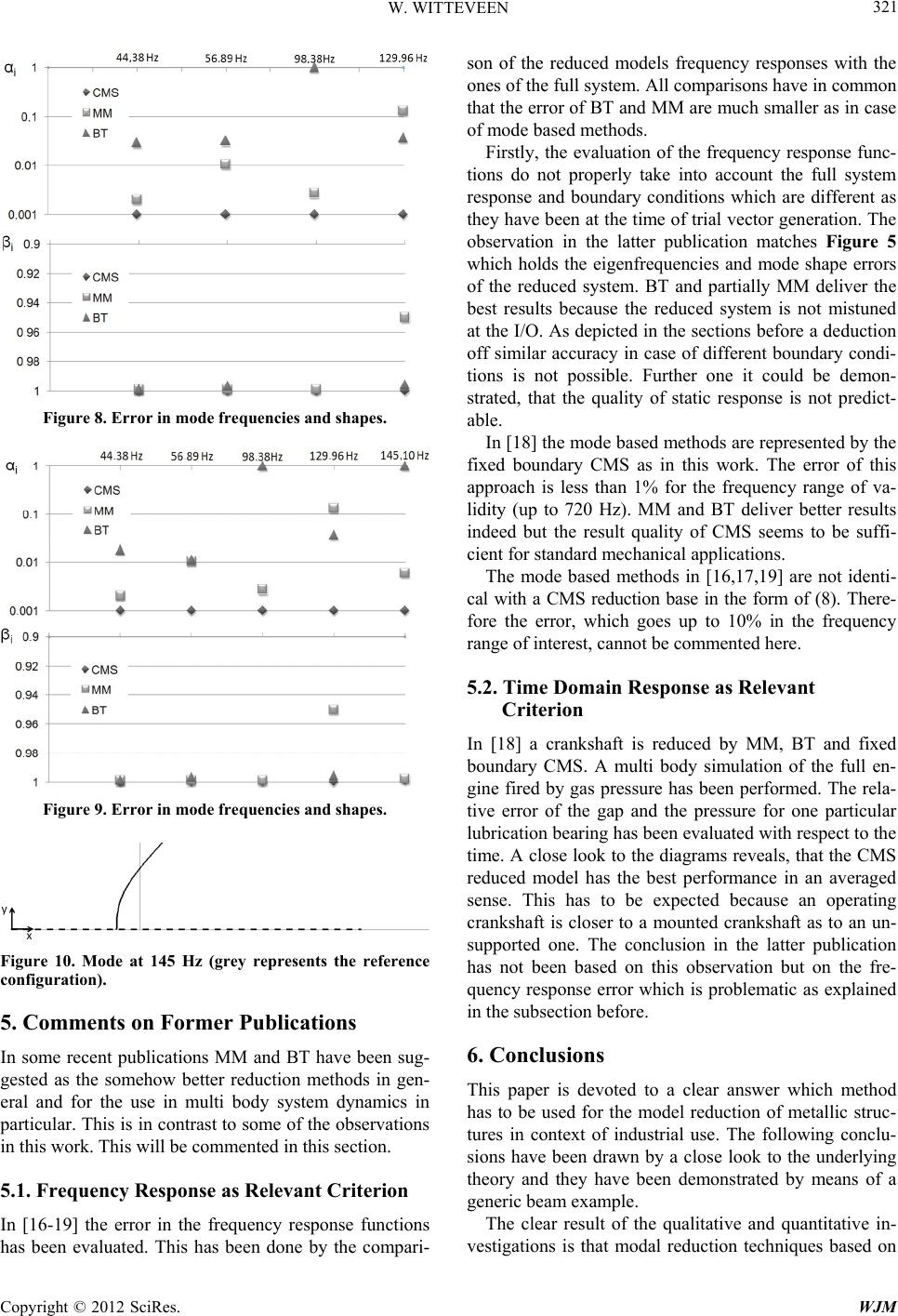

W. WITTEVEEN
321
Figure 8. Error in mode frequencies and shape s.
Figure 9. Error in mode frequencies and shape s.
Figure 10. Mode at 145 Hz (grey represents the reference
configuration).
5. Comments on Former Publications
In some recent publications MM and BT have been sug-
gested as the somehow better reduction methods in gen-
eral and for the use in multi body system dynamics in
particular. This is in contrast to some of the observations
in this work. This will be commented in this section.
5.1. Frequency Response as Relevant Criterion
In [16-19] the error in the frequency response functions
has been evaluated. This has been done by the compari-
son of the reduced models frequency responses with the
ones of the full system. All comparisons have in common
that the error of BT and MM are much smaller as in case
of mode based methods.
Firstly, the evaluation of the frequency response func-
tions do not properly take into account the full system
response and boundary conditions which are different as
they have been at the time of trial vector generation. The
observation in the latter publication matches Figure 5
which holds the eigenfrequencies and mode shape errors
of the reduced system. BT and partially MM deliver the
best results because the reduced system is not mistuned
at the I/O. As depicted in the sections before a deduction
off similar accuracy in case of different boundary condi-
tions is not possible. Further one it could be demon-
strated, that the quality of static response is not predict-
able.
In [18] the mode based methods are represented by the
fixed boundary CMS as in this work. The error of this
approach is less than 1% for the frequency range of va-
lidity (up to 720 Hz). MM and BT deliver better results
indeed but the result quality of CMS seems to be suffi-
cient for standard mechanical applications.
The mode based methods in [16,17,19] are not identi-
cal with a CMS reduction base in the form of (8). There-
fore the error, which goes up to 10% in the frequency
range of interest, cannot be commented here.
5.2. Time Domain Response as Relevant
Criterion
In [18] a crankshaft is reduced by MM, BT and fixed
boundary CMS. A multi body simulation of the full en-
gine fired by gas pressure has been performed. The rela-
tive error of the gap and the pressure for one particular
lubrication bearing has been evaluated with respect to the
time. A close look to the diagrams reveals, that the CMS
reduced model has the best performance in an averaged
sense. This has to be expected because an operating
crankshaft is closer to a mounted crankshaft as to an un-
supported one. The conclusion in the latter publication
has not been based on this observation but on the fre-
quency response error which is problematic as explained
in the subsection before.
6. Conclusions
This paper is devoted to a clear answer which method
has to be used for the model reduction of metallic struc-
tures in context of industrial use. The following conclu-
sions have been drawn by a close look to the underlying
theory and they have been demonstrated by means of a
generic beam example.
The clear result of the qualitative and quantitative in-
vestigations is that modal reduction techniques based on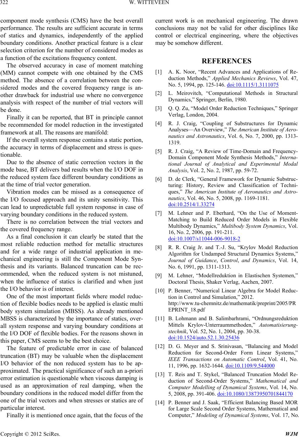

W. WITTEVEEN
322
component mode synthesis (CMS) have the best overall
performance. The results are sufficient accurate in terms
of statics and dynamics, independently of the applied
boundary conditions. Another practical feature is a clear
selection criterion for the number of considered modes as
a function of the excitations frequency content.
The observed accuracy in case of moment matching
(MM) cannot compete with one obtained by the CMS
method. The absence of a correlation between the con-
sidered modes and the covered frequency range is an-
other drawback for industrial use where no convergence
analysis with respect of the number of trial vectors will
be done.
Finally it can be reported, that BT in principle cannot
be recommended for model reduction in the investigated
framework at all. The reasons are manifold:
If the overall system response contains a static portion,
the accuracy in terms of displacement and stress is ques-
tionable.
Due to the absence of static correction vectors in the
mode base, BT delivers bad results when the I/O DOF in
the reduced system face different boundary conditions as
at the time of trial vector generation.
Vibration modes can be missed as a consequence of
the I/O focused approach and its unity sensitivity. This
can lead to unpredictable full system response in case of
varying boundary conditions in the reduced system.
There is no correlation between the trial vectors and
the covered frequency range.
As a final conclusion it can clearly be stated that the
most reliable reduction method for metallic structures
and for a wide range of industrial application in me-
chanical engineering is still the Component Mode Syn-
thesis and its variants. Balanced truncation can be rec-
ommended, when the reduced system is not mistuned,
when the influence of statics is clarified and when just
the I/O behavior is of interest.
One of the most important fields where model reduc-
tion of flexible bodies needs to be applied is elastic multi
body system simulation (MBSS). As already mentioned
MBSS is characterized by the importance of statics, over-
all system response and varying boundary conditions at
the I/O DOF of flexible bodies. For the reasons shown in
this paper, CMS seems to be the best choice.
The feature of predictable error in case of balanced
truncation (BT) may be valuable when the displacement
I/O behavior of the non reduced system has to be ap-
proximated. The practical significance of such an a-priori
error estimation is questionable when viscous damping is
used as an approximation of real damping, when the
boundary conditions in the reduced model differ from the
one of the trial vectors and when stresses or statics are of
particular interest.
Finally it is mentioned once again, that the focus of the
current work is on mechanical engineering. The drawn
conclusions may not be valid for other disciplines like
control or electrical engineering, where the objectives
may be somehow different.
REFERENCES
[1] A. K. Noor, “Recent Advances and Applications of Re-
duction Methods,” Applied Mechanics Reviews, Vol. 47,
No. 5, 1994, pp. 125-146. doi:10.1115/1.3111075
[2] L. Meirovitch, “Computational Methods in Structural
Dynamics,” Springer, Berlin, 1980.
[3] Q. Q. Zu, “Model Order Reduction Techniques,” Springer
Verlag, London, 2004.
[4] R. J. Craig, “Coupling of Substructures for Dynamic
Analyses—An Overview,” The American Institute of Aero-
nautics and Astronautics, Vol. 6, No. 7, 2000, pp. 1313-
1319.
[5] R. J. Craig, “A Review of Time-Domain and Frequency-
Domain Component Mode Synthesis Methods,” Interna-
tional Journal of Analytical and Experimental Modal
Analysis, Vol. 2, No. 2, 1987, pp. 59-72.
[6] D. de Clerk, “General Framework for Dynamic Substruc-
turing: History, Review and Classification of Techni-
ques,” The American Institute of Aeronautics and Astro-
nautics, Vol. 46, No. 5, 2008, pp. 1169-1181.
doi:10.2514/1.33274
[7] M. Lehner and P. Eberhard, “On the Use of Moment-
Matching to Build Reduced Order Models in Flexible
Multibody Dynamics,” Multibody System Dynamics, Vol.
16, No. 2, 2006, pp. 191-211.
doi:10.1007/s11044-006-9018-2
[8] R. R. Craig Jr. and T.-J. Su, “Krylov Model Reduction
Algorithm for Undamped Structural Dynamics Systems,”
Journal of Guidance, Control, and Dynamics, Vol. 14,
No. 6, 1991, pp. 1311-1313.
[9] M. Lehner, “Modellreduktion in Elastischen Systemen,”
Doctoral Thesis, Shaker Verlag, Aachen, 2007.
[10] P. Benner, “Numerical Linear Algebra for Model Reduc-
tion in Control and Simulation,” 2012.
http://www.tu-chemnitz.de/mathematik/preprint/2005/PR
EPRINT_18.pdf
[11] B. Lohmann and B. Salimbarhrami, “Ordnungsreduktion
Mittels Krylov-Unterraummethoden,” Automatisierung-
stechnik, Vol. 52, No. 1, 2004, pp. 30-38.
doi:10.1524/auto.52.1.30.25436
[12] D. G. Meyer and S. Srinivasan, “Balancing and Model
Reduction for Second-Order Form Linear Systems,”
IEEE Transactions on Automatic Control, Vol. 41, No.
11, 1996, pp. 1632-1644. doi:10.1109/9.544000
[13] T. Reis and T. Stykel, “Balanced Truncation Model Re-
duction of Second-Order Systems,” Mathematical and
Computer Modelling of Dynamical Systems, Vol. 14, No.
5, 2008, pp. 391-406. doi:10.1080/13873950701844170
[14] P. Benner and J. Saak, “Efficient Balancing Based MOR
for Large Scale Second Order Systems, Mathematical and
Computer,” Modeling of Dynamical Systems, Vol. 17, No.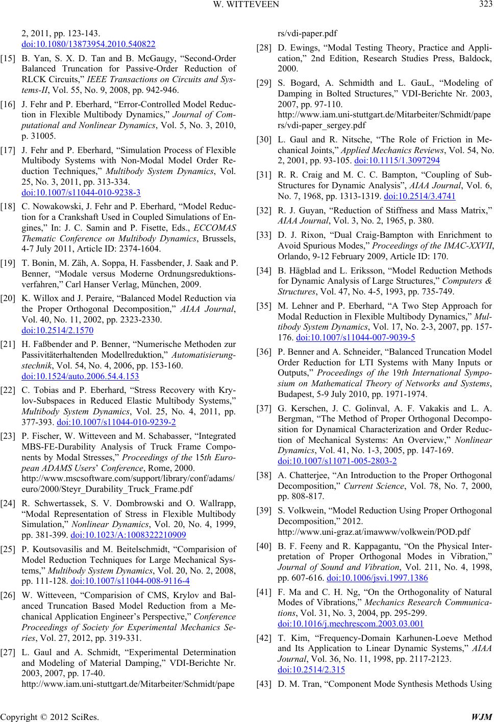

W. WITTEVEEN
323
2, 2011, pp. 123-143.
doi:10.1080/13873954.2010.540822
[15] B. Yan, S. X. D. Tan and B. McGaugy, “Second-Order
Balanced Truncation for Passive-Order Reduction of
RLCK Circuits,” IEEE Transactions on Circuits and Sys-
tems-II, Vol. 55, No. 9, 2008, pp. 942-946.
[16] J. Fehr and P. Eberhard, “Error-Controlled Model Reduc-
tion in Flexible Multibody Dynamics,” Journal of Com-
putational and Nonlinear Dynamics, Vol. 5, No. 3, 2010,
p. 31005.
[17] J. Fehr and P. Eberhard, “Simulation Process of Flexible
Multibody Systems with Non-Modal Model Order Re-
duction Techniques,” Multibody System Dynamics, Vol.
25, No. 3, 2011, pp. 313-334.
doi:10.1007/s11044-010-9238-3
[18] C. Nowakowski, J. Fehr and P. Eberhard, “Model Reduc-
tion for a Crankshaft Used in Coupled Simulations of En-
gines,” In: J. C. Samin and P. Fisette, Eds., ECCOMAS
Thematic Conference on Multibody Dynamics, Brussels,
4-7 July 2011, Article ID: 2374-1604.
[19] T. Bonin, M. Zäh, A. Soppa, H. Fassbender, J. Saak and P.
Benner, “Modale versus Moderne Ordnungsreduktions-
verfahren,” Carl Hanser Verlag, München, 2009.
[20] K. Willox and J. Peraire, “Balanced Model Reduction via
the Proper Orthogonal Decomposition,” AIAA Journal,
Vol. 40, No. 11, 2002, pp. 2323-2330.
doi:10.2514/2.1570
[21] H. Faßbender and P. Benner, “Numerische Methoden zur
Passivitäterhaltenden Modellreduktion,” Automatisierung-
stechnik, Vol. 54, No. 4, 2006, pp. 153-160.
doi:10.1524/auto.2006.54.4.153
[22] C. Tobias and P. Eberhard, “Stress Recovery with Kry-
lov-Subspaces in Reduced Elastic Multibody Systems,”
Multibody System Dynamics, Vol. 25, No. 4, 2011, pp.
377-393. doi:10.1007/s11044-010-9239-2
[23] P. Fischer, W. Witteveen and M. Schabasser, “Integrated
MBS-FE-Durability Analysis of Truck Frame Compo-
nents by Modal Stresses,” Proceedings of the 15th Euro-
pean ADAMS Users’ Conference, Rome, 2000.
http://www.mscsoftware.com/support/library/conf/adams/
euro/2000/Steyr_Durability_Truck_Frame.pdf
[24] R. Schwertassek, S. V. Dombrowski and O. Wallrapp,
“Modal Representation of Stress in Flexible Multibody
Simulation,” Nonlinear Dynamics, Vol. 20, No. 4, 1999,
pp. 381-399. doi:10.1023/A:1008322210909
[25] P. Koutsovasilis and M. Beitelschmidt, “Comparision of
Model Reduction Techniques for Large Mechanical Sys-
tems,” Multibody System Dynamics, Vol. 20, No. 2, 2008,
pp. 111-128. doi:10.1007/s11044-008-9116-4
[26] W. Witteveen, “Comparision of CMS, Krylov and Bal-
anced Truncation Based Model Reduction from a Me-
chanical Application Engineer’s Perspective,” Conference
Proceedings of Society for Experimental Mechanics Se-
ries, Vol. 27, 2012, pp. 319-331.
[27] L. Gaul and A. Schmidt, “Experimental Determination
and Modeling of Material Damping,” VDI-Berichte Nr.
2003, 2007, pp. 17-40.
http://www.iam.uni-stuttgart.de/Mitarbeiter/Schmidt/pape
rs/vdi-paper.pdf
[28] D. Ewings, “Modal Testing Theory, Practice and Appli-
cation,” 2nd Edition, Research Studies Press, Baldock,
2000.
[29] S. Bogard, A. Schmidth and L. GauL, “Modeling of
Damping in Bolted Structures,” VDI-Berichte Nr. 2003,
2007, pp. 97-110.
http://www.iam.uni-stuttgart.de/Mitarbeiter/Schmidt/pape
rs/vdi-paper_sergey.pdf
[30] L. Gaul and R. Nitsche, “The Role of Friction in Me-
chanical Joints,” Applied Mechanics Reviews, Vol. 54, No.
2, 2001, pp. 93-105. doi:10.1115/1.3097294
[31] R. R. Craig and M. C. C. Bampton, “Coupling of Sub-
Structures for Dynamic Analysis”, AIAA Journal, Vol. 6,
No. 7, 1968, pp. 1313-1319. doi:10.2514/3.4741
[32] R. J. Guyan, “Reduction of Stiffness and Mass Matrix,”
AIAA Journal, Vol. 3, No. 2, 1965, p. 380.
[33] D. J. Rixon, “Dual Craig-Bampton with Enrichment to
Avoid Spurious Modes,” Proceedings of the IMAC-XXVII,
Orlando, 9-12 February 2009, Article ID: 170.
[34] B. Hägblad and L. Eriksson, “Model Reduction Methods
for Dynamic Analysis of Large Structures,” Computers &
Structures, Vol. 47, No. 4-5, 1993, pp. 735-749.
[35] M. Lehner and P. Eberhard, “A Two Step Approach for
Modal Reduction in Flexible Multibody Dynamics,” Mul-
tibody System Dynamics, Vol. 17, No. 2-3, 2007, pp. 157-
176. doi:10.1007/s11044-007-9039-5
[36] P. Benner and A. Schneider, “Balanced Truncation Model
Order Reduction for LTI Systems with Many Inputs or
Outputs,” Proceedings of the 19th International Sympo-
sium on Mathematical Theory of Networks and Systems,
Budapest, 5-9 July 2010, pp. 1971-1974.
[37] G. Kerschen, J. C. Golinval, A. F. Vakakis and L. A.
Bergman, “The Method of Proper Orthogonal Decompo-
sition for Dynamical Characterization and Order Reduc-
tion of Mechanical Systems: An Overview,” Nonlinear
Dynamics, Vol. 41, No. 1-3, 2005, pp. 147-169.
doi:10.1007/s11071-005-2803-2
[38] A. Chatterjee, “An Introduction to the Proper Orthogonal
Decomposition,” Current Science, Vol. 78, No. 7, 2000,
pp. 808-817.
[39] S. Volkwein, “Model Reduction Using Proper Orthogonal
Decomposition,” 2012.
http://www.uni-graz.at/imawww/volkwein/POD.pdf
[40] B. F. Feeny and R. Kappagantu, “On the Physical Inter-
pretation of Proper Orthogonal Modes in Vibration,”
Journal of Sound and Vibration, Vol. 211, No. 4, 1998,
pp. 607-616. doi:10.1006/jsvi.1997.1386
[41] F. Ma and C. H. Ng, “On the Orthogonality of Natural
Modes of Vibrations,” Mechanics Research Communica-
tions, Vol. 31, No. 3, 2004, pp. 295-299.
doi:10.1016/j.mechrescom.2003.03.001
[42] T. Kim, “Frequency-Domain Karhunen-Loeve Method
and Its Application to Linear Dynamic Systems,” AIAA
Journal, Vol. 36, No. 11, 1998, pp. 2117-2123.
doi:10.2514/2.315
[43] D. M. Tran, “Component Mode Synthesis Methods Using

W. WITTEVEEN
324
Interface Modes. Application to Structures with Cyclic
Symmetry,” Computers and Structures, Vol. 79, No. 2,
2001, pp. 209-222. doi:10.1016/S0045-7949(00)00121-8
[44] E. Balmes, “Use of Generalized Interface Degrees of
Freedom in Component Mode Synthesis,” Proceedings of
IMAC XIV Conference, Milwaukee, 12-15 February 1996,
pp. 204-210.
[45] W. Witteveen and H. Irschik, “Efficient Mode-Based
Computational Approach for Jointed Structures: Joint In-
terface Modes,” AIAA Journal, Vol. 47, No. 1, 2009, pp.
252-263. doi:10.2514/1.38436
[46] MD R3 Nastran, 2008. www.mscsoftware.com
[47] Scilab, Version 5.3.0. www.scilab.org
[48] R. J. Allemang and D. L. Brown, “A Correlation Coeffi-
cient for Modal Vector Analysis,” Proceedings of the 1st
International Modal Analysis Conference (IMAC I), Or-
lando, 8-10 November 1982, pp. 110-116.
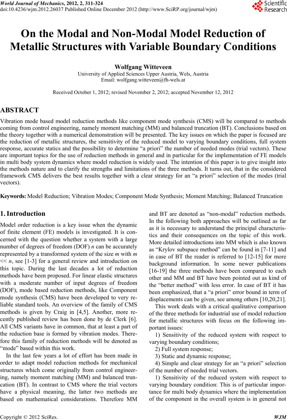