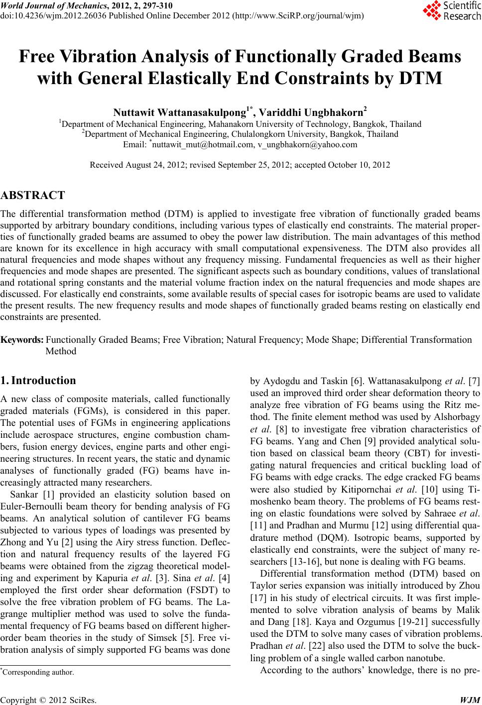
World Journal of Mechanics, 2012, 2, 297-310
doi:10.4236/wjm.2012.26036 Published Online December 2012 (http://www.SciRP.org/journal/wjm)
Free Vibration Analysis of Functionally Graded Beams
with General Elastically End Constraints by DTM
Nuttawit Wattanasakulpong1*, Variddhi Ungbhakorn2
1Department of Mechanical Engineering, Mahanakorn University of Technology, Bangkok, Thailand
2Department of Mechanical Engineering, Chulalongkorn University, Bangkok, Thailand
Received August 24, 2012; revised September 25, 2012; accepted October 10, 2012
ABSTRACT
The differential transformation method (DTM) is applied to investigate free vibration of functionally graded beams
supported by arbitrary boundary conditions, including various types of elastically end constraints. The material proper-
ties of functionally graded beams are assumed to obey the power law distribution. The main advantages of this method
are known for its excellence in high accuracy with small computational expensiveness. The DTM also provides all
natural frequencies and mode shapes without any frequency missing. Fundamental frequencies as well as their higher
frequencies and mode shapes are presented. The significant aspects such as boundary conditions, values of translational
and rotational spring constants and the material volume fraction index on the natural frequencies and mode shapes are
discussed. For elastically end constraints, some available results of special cases for isotropic beams are used to validate
the present results. The new frequency results and mode shapes of functionally graded beams resting on elastically end
constraints are presented.
Keywords: Functionally Graded Beams; Free Vibration; Natural Frequency; Mode Shape; Differential Transformation
Method
1. Introduction
A new class of composite materials, called functionally
graded materials (FGMs), is considered in this paper.
The potential uses of FGMs in engineering applications
include aerospace structures, engine combustion cham-
bers, fusion energy devices, engine parts and other engi-
neering structures. In recent years, the static and dynamic
analyses of functionally graded (FG) beams have in-
creasingly attracted many researchers.
Sankar [1] provided an elasticity solution based on
Euler-Bernoulli beam theory for bending analysis of FG
beams. An analytical solution of cantilever FG beams
subjected to various types of loadings was presented by
Zhong and Yu [2] using the Airy stress function. Deflec-
tion and natural frequency results of the layered FG
beams were obtained from the zigzag theoretical model-
ing and experiment by Kapuria et al. [3]. Sina et al. [4]
employed the first order shear deformation (FSDT) to
solve the free vibration problem of FG beams. The La-
grange multiplier method was used to solve the funda-
mental frequency of FG beams based on different higher-
order beam theories in the study of Simsek [5]. Free vi-
bration analysis of simply supported FG beams was done
by Aydogdu and Taskin [6]. Wattanasakulpong et al. [7]
used an improved third order shear deformation theory to
analyze free vibration of FG beams using the Ritz me-
thod. The finite element method was used by Alshorbagy
et al. [8] to investigate free vibration characteristics of
FG beams. Yang and Chen [9] provided analytical solu-
tion based on classical beam theory (CBT) for investi-
gating natural frequencies and critical buckling load of
FG beams with edge cracks. The edge cracked FG beams
were also studied by Kitipornchai et al. [10] using Ti-
moshenko beam theory. The problems of FG beams rest-
ing on elastic foundations were solved by Sahraee et al.
[11] and Pradhan and Murmu [12] using differential qua-
drature method (DQM). Isotropic beams, supported by
elastically end constraints, were the subject of many re-
searchers [13-16], but none is dealing with FG beams.
Differential transformation method (DTM) based on
Taylor series expansion was initially introduced by Zhou
[17] in his study of electrical circuits. It was first imple-
mented to solve vibration analysis of beams by Malik
and Dang [18]. Kaya and Ozgumus [19-21] successfully
used the DTM to solve many cases of vibration problems.
Pradhan et al. [22] also used the DTM to solve the buck-
ling problem of a single walled carbon nanotube.
According to the authors’ knowledge, there is no pre-
*Corresponding author.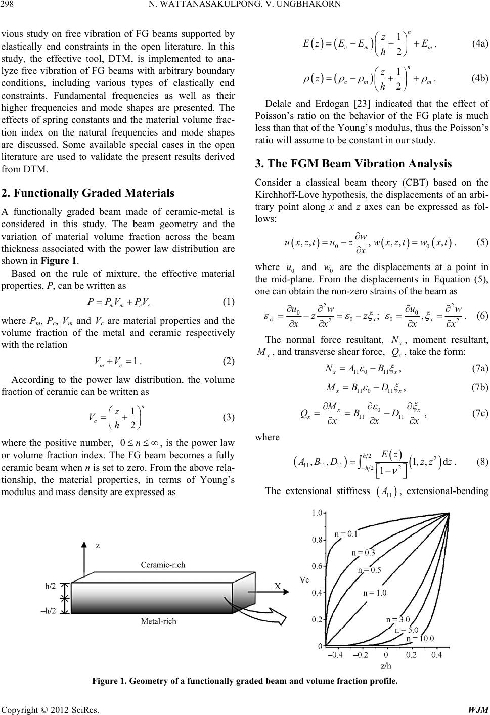

N. WATTANASAKULPONG, V. UNGBHAKORN
298
vious study on free vibration of FG beams supported by
elastically end constraints in the open literature. In this
study, the effective tool, DTM, is implemented to ana-
lyze free vibration of FG beams with arbitrary boundary
conditions, including various types of elastically end
constraints. Fundamental frequencies as well as their
higher frequencies and mode shapes are presented. The
effects of spring constants and the material volume frac-
tion index on the natural frequencies and mode shapes
are discussed. Some available special cases in the open
literature are used to validate the present results derived
from DTM.
2. Functionally Graded Materials
A functionally graded beam made of ceramic-metal is
considered in this study. The beam geometry and the
variation of material volume fraction across the beam
thickness associated with the power law distribution are
shown in Figure 1.
Based on the rule of mixture, the effective material
properties, P, can be written as
mm cc
PPV PV (1)
where Pm, Pc, Vm and Vc are material properties and the
volume fraction of the metal and ceramic respectively
with the relation
1
mc
VV. (2)
According to the power law distribution, the volume
fraction of ceramic can be written as
1
2
n
c
z
Vh




(3)
where the positive number, 0n

, is the power law
or volume fraction index. The FG beam becomes a fully
ceramic beam when n is set to zero. From the above rela-
tionship, the material properties, in terms of Young’s
modulus and mass density are expressed as


1
2
n
cm m
z
EzE EE
h

 

 , (4a)


1
2
n
cm m
z
zh

 

 

 . (4b)
Delale and Erdogan [23] indicated that the effect of
Poisson’s ratio on the behavior of the FG plate is much
less than that of the Young’s modulus, thus the Poisson’s
ratio will assume to be constant in our study.
3. The FGM Beam Vibration Analysis
Consider a classical beam theory (CBT) based on the
Kirchhoff-Love hypothesis, the displacements of an arbi-
trary point along x and z axes can be expressed as fol-
lows:
 
00
,,,,,,
w
uxztuzwxztw xt
x

 
. (5)
where 0
u and 0 w are the displacements at a point in
the mid-plane. From the displacements in Equation (5),
one can obtain the non-zero strains of the beam as
22
00
00
22
;,
xxx x
uu
ww
zz
xx
x
x




 


. (6)
The normal force resultant,
x
N, moment resultant,
x
M
, and transverse shear force,
x
Q, take the form:
11 011
x
x
NA B



, (7a)
11 011
x
x
MB D



, (7b)
0
11 11
x
x
x
M
QBD
x
xx




 


, (7c)
where



22
11 11112
2
,,1,, d
1
h
h
Ez
A
BDzz z





. (8)
The extensional stiffness

11
A
, extensional-bending
Figure 1. Geometry of a functionally graded beam and volume fraction profile.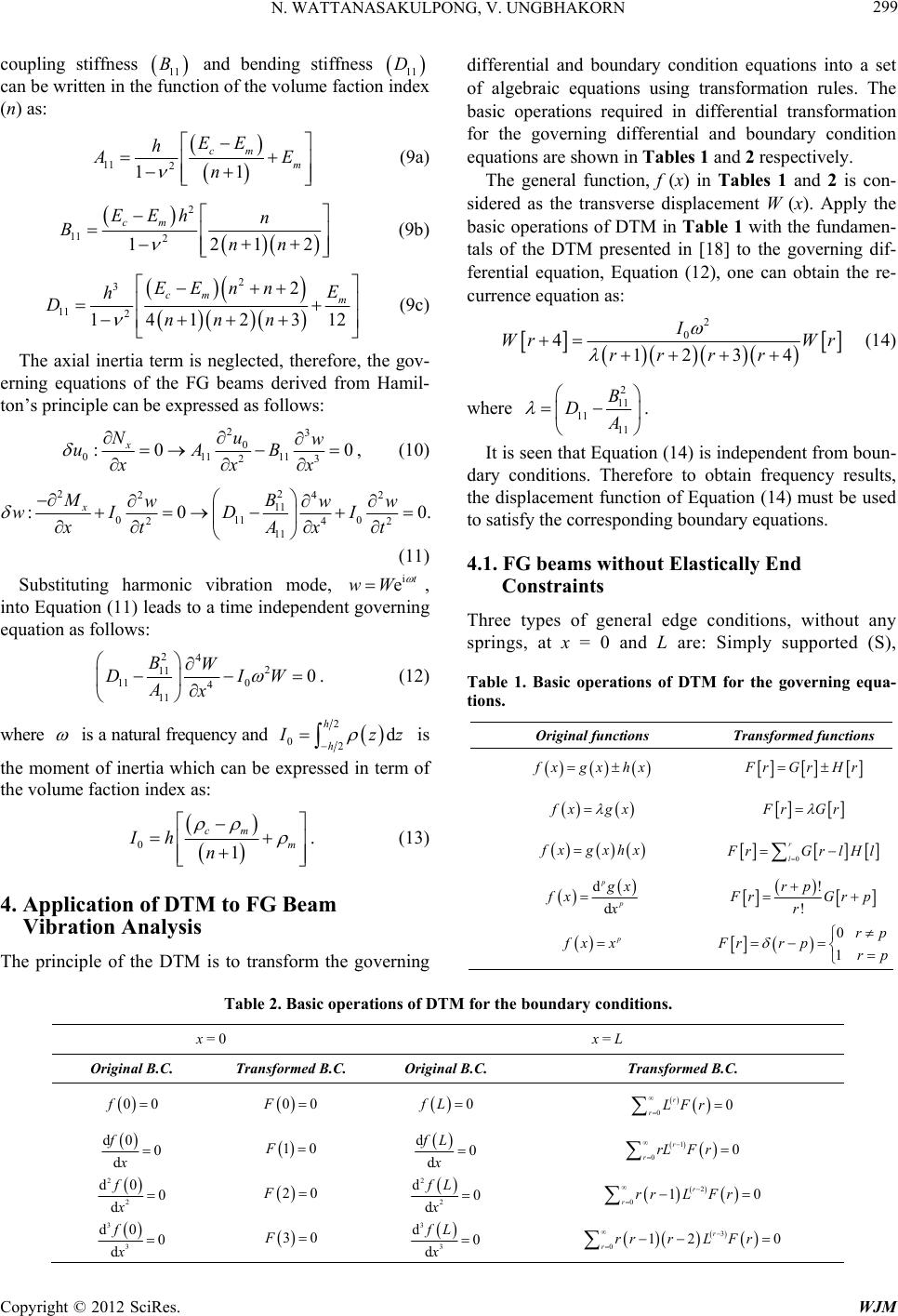

N. WATTANASAKULPONG, V. UNGBHAKORN
299
coupling stiffness

11
B and bending stiffness


11
D
can be written in the function of the volume faction index
(n) as:


11 21
1
cm
m
EE
h
A
E
n

 





(9a)

 
2
11 221 2
1
cm
EEh n
Bnn







(9b)



 
2
3
11 2
2
41 2312 1
cm m
EE nnE
h
Dnn n





 


(9c)
The axial inertia term is neglected, therefore, the gov-
erning equations of the FG beams derived from Hamil-
ton’s principle can be expressed as follows:
23
0
01111
23
:0 0
x
Nu w
uAB
xxx

 
 

, (10)
22 242
11
0110
242
11
:0 0.
x
MB www
wI DI
xA
txt

  
 



(11)
Substituting harmonic vibration mode, i et wW

,
into Equation (11) leads to a time independent governing
equation as follows:
24
2 11
11 0
4
11
0
BW
DIW
Ax






 . (12)
where

is a natural frequency and

2
02d
h
h
I
zz 

 is
the moment of inertia which can be expressed in term of
the volume faction index as:


01
cm
m
Ih n


 





. (13)
4. Application of DTM to FG Beam
Vibration Analysis
The principle of the DTM is to transform the governing
differential and boundary condition equations into a set
of algebraic equations using transformation rules. The
basic operations required in differential transformation
for the governing differential and boundary condition
equations are shown in Tables 1 and 2 respectively.
The general function, f (x) in Tables 1 and 2 is con-
sidered as the transverse displacement W (x). Apply the
basic operations of DTM in Table 1 with the fundamen-
tals of the DTM presented in [18] to the governing dif-
ferential equation, Equation (12), one can obtain the re-
currence equation as:

  

2
0
41234
I
Wr Wr
rrr r


   (14)
where
2
11
11
11
B
D
A





.
It is seen that Equation (14) is independent from boun-
dary conditions. Therefore to obtain frequency results,
the displacement function of Equation (14) must be used
to satisfy the corresponding boundary equations.
4.1. FG beams without Elastically End
Constraints
Three types of general edge conditions, without any
springs, at x = 0 and L are: Simply supported (S),
Table 1. Basic operations of DTM for the governing equa-
tions.
Original functions Transformed functions






f
xgxhx






F
rGrHr




f
xgx  




F
rGr  






f
xgxhx

0
r
l
F
rGrlHl






d
d
p
p
g
x
fx x 



!
!
rp
F
rGrp
r




p
f
xx

 
0
1
rp
Frr prp 






Table 2. Basic operations of DTM for the boundary c onditions.
x = 0 x = L
Original B.C. Transforme d B.C. Original B.C. Transforme d B.C.

00f

00F


0fL



00
r
rLFr




d0 0
d
f
x

10F


d0
d
fL
x



1
00
r
rrLF r




2
2
d00
d
f
x

20F


2
2
d0
d
fL
x




2
010
r
rrrL Fr






3
3
d00
d
f
x

30F


3
3
d0
d
fL
x




3
012 0
r
rrrrL Fr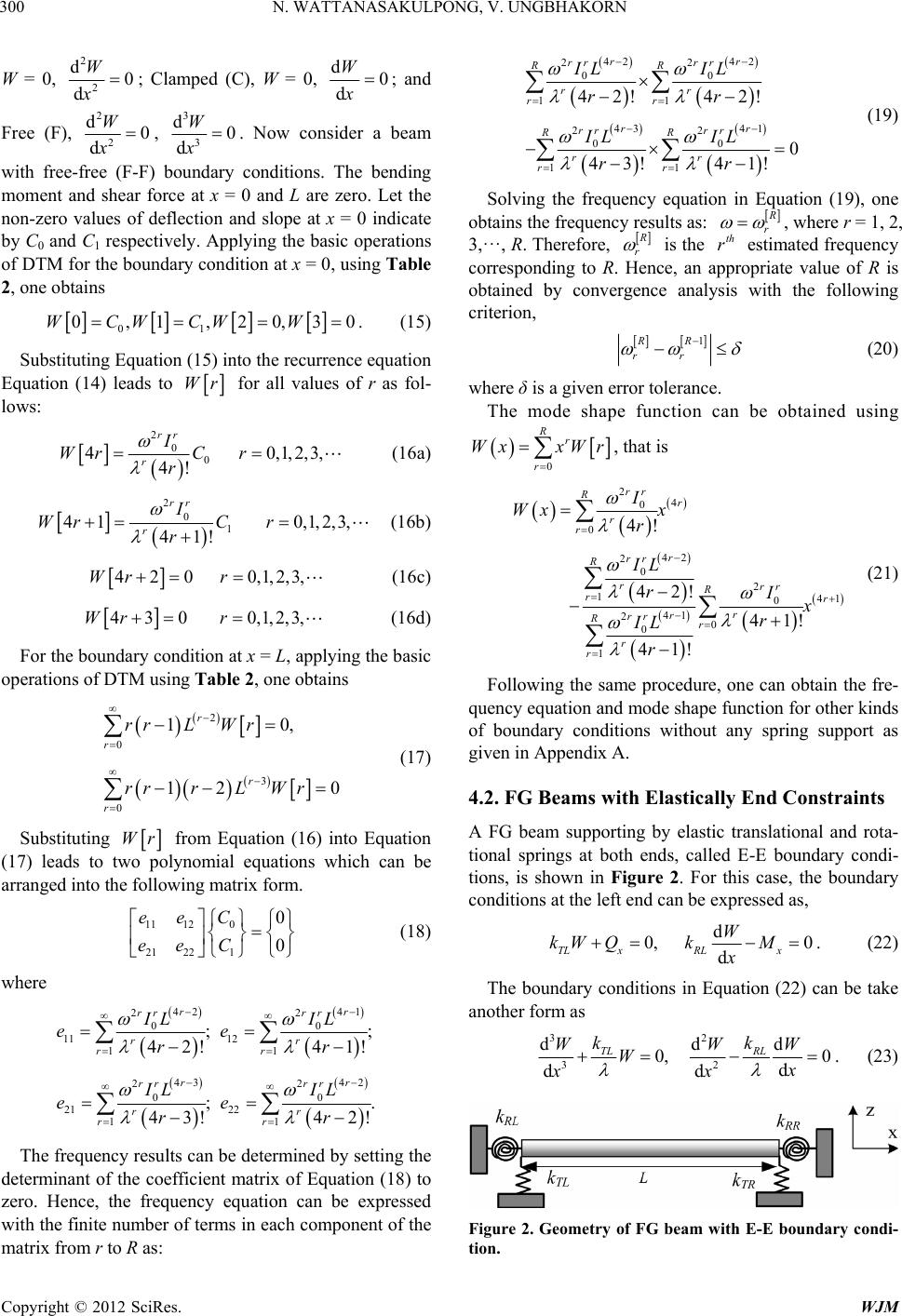






N. WATTANASAKULPONG, V. UNGBHAKORN
300
W = 0,
2
2
d0
d
W
x; Clamped (C), W = 0, d0
d
W
x

; and
Free (F),
2
2
d0
d
W
x,
3
3
d0
d
W
x. Now consider a beam
with free-free (F-F) boundary conditions. The bending
moment and shear force at x = 0 and L are zero. Let the
non-zero values of deflection and slope at x = 0 indicate
by C0 and C1 respectively. Applying the basic operations
of DTM for the boundary condition at x = 0, using Table
2, one obtains








01
0,1,20,30WCWCWW. (15)
Substituting Equation (15) into the recurrence equation
Equation (14) leads to


Wr for all values of r as fol-
lows:


2
0
0
40,1,2,3,
4!
rr
r
I
WrC r
r


 (16a)


2
0
1
410,1,2,3,
41!
rr
r
I
WrC r
r


 
 (16b)


420 0,1,2,3,Wr r  (16c)


430 0,1,2,3,Wr r  (16d)
For the boundary condition at x = L, applying the basic
operations of DTM using Table 2, one obtains



 


2
0
3
0
10,
12 0
r
r
r
r
rrL Wr
rrrLWr





 


(17)
Substituting


Wr from Equation (16) into Equation
(17) leads to two polynomial equations which can be
arranged into the following matrix form.
11 120
21 221
0
0
ee C
ee C
 




(18)
where








42 41
22
00
11 12
11
43 42
22
00
21 22
11
;;
42! 41!
;.
43! 42!
rr
rr rr
rr
rr
rr
rrrr
rr
rr
IL IL
ee
rr
IL IL
ee
rr
















The frequency results can be determined by setting the
determinant of the coefficient matrix of Equation (18) to
zero. Hence, the frequency equation can be expressed
with the finite number of terms in each component of the
matrix from r to R as:









42 42
22
00
11
43 41
22
00
11
42! 42!
0
43! 41!
rr
rr rr
RR
rr
rr
rr
rr rr
RR
rr
rr
IL IL
rr
IL IL
rr















(19)
Solving the frequency equation in Equation (19), one
obtains the frequency results as:

R
r

 , where r = 1, 2,
3,···, R. Therefore,

R
r

is the th r estimated frequency
corresponding to R. Hence, an appropriate value of R is
obtained by convergence analysis with the following
criterion,
 
1RR
rr




 (20)
where δ is a given error tolerance.
The mode shape function can be obtained using
 
0
Rr
r
Wx xWr

, that is
 







2
4
0
0
42
2
0
2
141
0
41
20
0
1
4!
42!
41!
41!
rr
Rr
r
r
r
rr
R
rrr
R
rr
r
r
rr
Rr
r
r
I
Wx x
r
IL
rIx
r
IL
r




















(21)
Following the same procedure, one can obtain the fre-
quency equation and mode shape function for other kinds
of boundary conditions without any spring support as
given in Appendix A.
4.2. FG Beams with Elastically End Constraints
A FG beam supporting by elastic translational and rota-
tional springs at both ends, called E-E boundary condi-
tions, is shown in Figure 2. For this case, the boundary
conditions at the left end can be expressed as,
d
0, 0
d
TL xRLx
W
kW QkM
x

. (22)
The boundary conditions in Equation (22) can be take
another form as
32
32
ddd
0, 0
d dd
TL RL
kk WWW
Wx
xx 


. (23)
Figure 2. Geometry of FG beam with E-E boundary condi-
tion.

N. WATTANASAKULPONG, V. UNGBHAKORN
301
Where kTL and kRL are the translational spring constant
(MN/m) and the rotational spring constant (MN·m/rad) at
the left end respectively. Let the non-zero values of de-
flection and slope at x = 0 be C0 and C1 respectively. Use
Table 2 to apply the basic operations of DTM for these
non-zero quantities at x = 0, one obtains




01
d
0,1
d
Wx
WWxCW C
x
  . (24)
The expressions for non-zero values of bending mo-
ment and shear force at x = 0 can be written as
 
0 1
2,3
26
TL RL kC
kC
WW


. (25)
To find []Wr for all values of r, the components in
Equations (24) and (25) are substituted into the recur-
rence Equation (14).


2
00
4,0,1, 2,3,.
4!
rr
r
IC
Wr r
r


 (26a)


2
00
4,0,1, 2,3,.
4!
rr
r
IC
Wr r
r


 (26b)


2
01
(1)
42 0,1,2,3,.
42!
rr
RL
r
IkC
Wr r
r



 
， (26c)


2
00
(1)
43 0,1,2,3,.
43!
rr
TL
r
Ik C
Wr r
r




， (26d)
At x = L, the boundary conditions are
d0, 0
d
RRxTR x
W
kMkWQ
x 
. (27)
They can be written as:
23
23
ddd
0, 0
d dd
RR TR
kk
WW W
W
x xx 
 . (28)
Similarly, applying the DTM to the boundary condi-
tions (28) yields





21
00
10
rr
RR
rr
k
rrLWrrL Wr







, (29a)
 




3
00
12 0
rr
TR
rr
k
rrrLWrLWr





 

.(29b)
Substituting


Wr from Equation (26) into Equation
(29) leads to two polynomial equations which can be
arranged into the following matrix form:
11 120
21 221
0
0
ppC
ppC
 



 
(30)
where:











42 41
22
00
11 1
11
41 42
22
00
12
00
42!41!
41! 42!
rr
rr rr
RR
rr
rr
rr
rr rr
TLRR TL
rr
rr
LI LI
pk
rr
LIL I
kkk
rr





























41 4
22
00
12 1
10
441
22
00
12
00
41!4!
4!4 1!
rr
rr rr
RR
rr
rr
rr
rr rr
RLRR RL
rr
rr
LI LI
pk
rr
LIL I
kkk
rr














 













43 4
22
00
21 1
10
443
22
00
12
00
43! 4!
4!4 3!
rr
rr rr
TR
rr
rr
rr
rr rr
TLTR TL
rr
rr
LI LI
pk
rr
LIL I
kkk
rr














 













42 41
22
00
22 1
10
414 2
22
00
12
10
42! 41!
.
41!42!
rr
rr rr
TR
rr
rr
rr
rr rr
RLTR RL
rr
rr
LI LI
pk
rr
LIL I
kkk
rr


















Similarly, set the determinant of the coefficient matrix
of Equation (30) to zero with finite number of terms, one
obtains the following frequency equation.


















42 414142
222 2
000 0
112
10
42 4141
222
000
11
42! 41!41!4 2!
42! 41! 4
rrr r
rr rrrrrr
RR
RRTLRR TL
rrrr
rr
rr r
rr rrrr
RL TR
rrr
LI LILILI
kkkk
rrrr
LI LILI
kk
rrr
 

 




 

 
 
   
 

 
 
 

 






















42 2
0
2
10
43434 4
2222
0000
211
10
41 41
22
0
1!4 2!
43! 43! 4! 4!
41!
rrr
RR
TR RLr
rr
rrrr
rrrrrr rr
RR
TR TLTRTL
rrrr
rr
rr
rr
RR RL
r
LI
kk r
LILILI LI
kkkk
rrrr
LI L
kk
r













 

   

  

 


  

















44
22
000
211
10
0
41! 4!4!
rr
rrrr rr
RR
RR RL
rrr
rr
ILILI
kk
rrr









 



(31)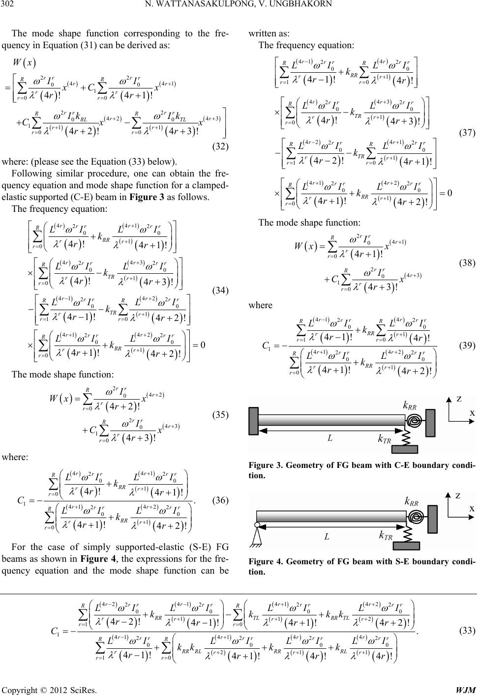

N. WATTANASAKULPONG, V. UNGBHAKORN
302
The mode shape function corresponding to the fre-
quency in Equation (31) can be derived as:











22
441
00
1
00
22
42 43
00
111
00
4!4 1!
42! 43!
rr rr
RR
rr
rr
rr
rr rr
RR
rr
RL TL
rr
rr
Wx
II
xC x
rr
Ik Ik
Cx x
rr






















(32)
where: (please see the Equation (33) below).
Following similar procedure, one can obtain the fre-
quency equation and mode shape function for a clamped-
elastic supported (C-E) beam in Figure 3 as follows.
The frequency equation:

















441
22
00
1
0
443
22
00
1
0
414 2
22
00
1
10
41 2
0
4! 41!
4! 43!
41!42!
41!
rr
rrrr
R
RR
rr
r
rr
rr rr
R
TR
rr
r
rr
rrrr
RR
TR
rr
rr
rrr
r
LIL I
k
rr
LIL I
k
rr
LIL I
k
rr
LI
r




















  







  

 
















42 2
0
1
0
0
42!
rrr
R
RR r
r
LI
kr










 



(34)
The mode shape function:
 



2
42
0
0
2
43
0
1
0
42!
43!
rr
Rr
r
r
rr
Rr
r
r
I
Wx x
r
I
Cx
r












(35)
where:










441
22
00
1
0
141 42
22
00
1
0
4! 41!
.
41!42!
rr
rrrr
R
RR
rr
r
rr rr rr
R
RR
rr
r
LIL I
k
rr
C
LI LI
k
rr
















 







(36)
For the case of simply supported-elastic (S-E) FG
beams as shown in Figure 4, the expressions for the fre-
quency equation and the mode shape function can be
written as:
The frequency equation:

















41 4
22
00
1
10
443
22
00
1
0
42 41
22
00
1
10
41 2
0
41!4!
4! 43!
42! 41!
41!
rr
rr rr
RR
RR
rr
rr
rr
rr rr
R
TR
rr
r
rr
rrrr
RR
TR
rr
rr
rrr
RR
r
LI LI
k
rr
LIL I
k
rr
LI LI
k
rr
LI
k
r



























 

 
















42 2
0
1
0
0
42!
rrr
R
r
r
LI
r















(37)
The mode shape function:
 



2
41
0
0
2
43
0
1
0
41!
43!
rr
Rr
r
r
rr
Rr
r
r
I
Wx x
r
I
Cx
r












(38)
where











41 4
22
00
1
10
141 42
22
00
1
0
41!4!
41!42!
rr
rr rr
RR
RR
rr
rr
rr
rr rr
R
RR
rr
r
LI LI
k
rr
C
LI LI
k
rr












 
 





(39)
Figure 3. Geometry of FG beam with C-E boundary condi-
tion.
Figure 4. Geometry of FG beam with S-E boundary condi-
tion.




















42 414142
222 2
000 0
112
10
141414 4
2222
0000
21
42!41!41!4 2!
41! 41! 4!
rrr r
rrrrrrrr
RR
RRTLRR TL
rrrr
rr
rrrr
rrrrrr r
RR RLRRRL
rrr
LI LILILI
kkkk
rrrr
C
LILILI LI
kkk k
rrr
 








 
   
 

 






1
10
.
4!
r
RR
r
rr r 







(33)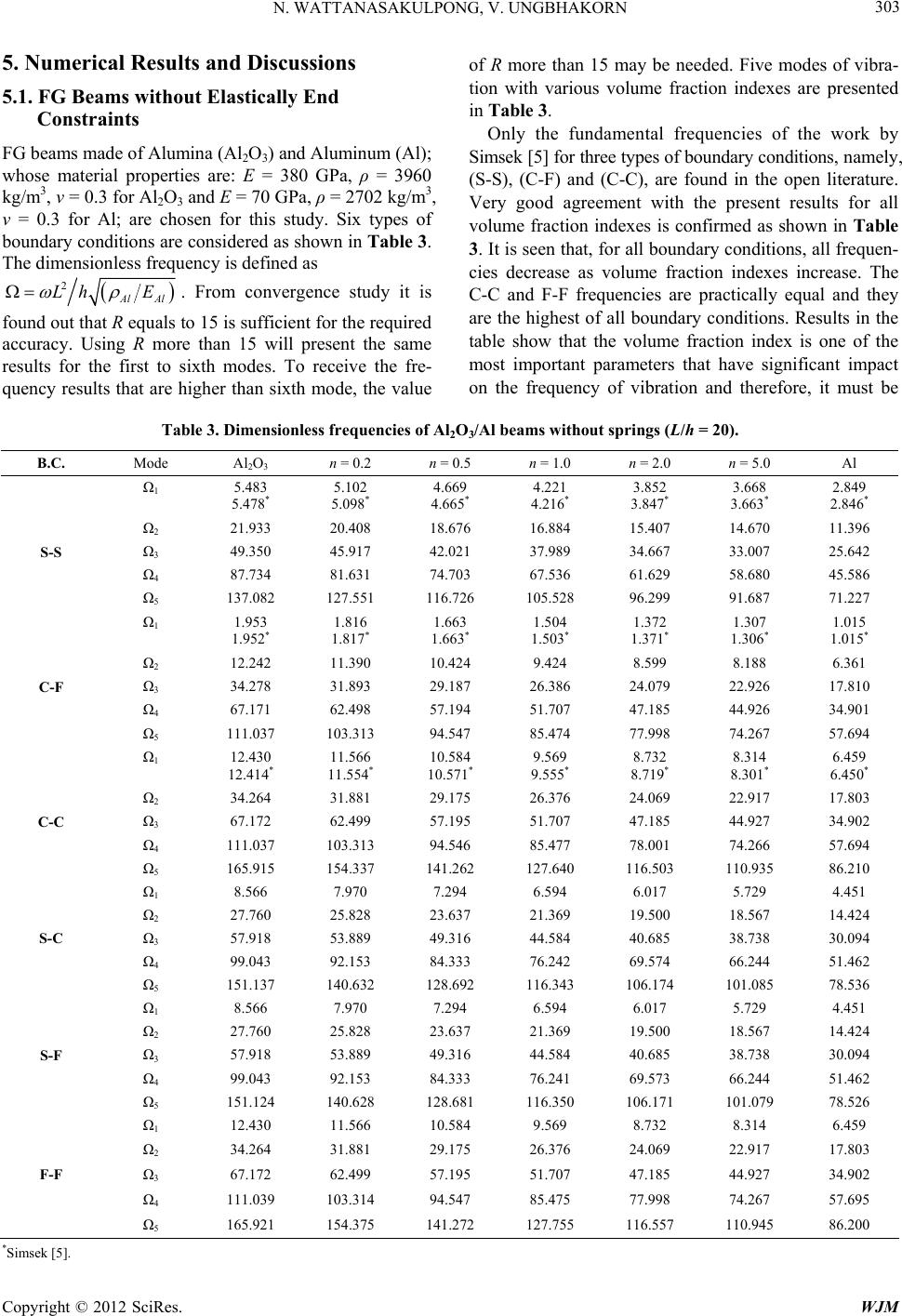

N. WATTANASAKULPONG, V. UNGBHAKORN
303
5. Numerical Results and Discussions
5.1. FG Beams without Elastically End
Constraints
FG beams made of Alumina (Al2O3) and Aluminum (Al);
whose material properties are: E = 380 GPa, ρ = 3960
kg/m3, ν = 0.3 for Al2O3 and E = 70 GPa, ρ = 2702 kg/m3,
ν = 0.3 for Al; are chosen for this study. Six types of
boundary conditions are considered as shown in Table 3.
The dimensionless frequency is defined as

2
Al Al
LhE   . From convergence study it is
found out that R equals to 15 is sufficient for the required
accuracy. Using R more than 15 will present the same
results for the first to sixth modes. To receive the fre-
quency results that are higher than sixth mode, the value
of R more than 15 may be needed. Five modes of vibra-
tion with various volume fraction indexes are presented
in Table 3.
Only the fundamental frequencies of the work by
Simsek [5] for three types of boundary conditions, namely,
(S-S), (C-F) and (C-C), are found in the open literature.
Very good agreement with the present results for all
volume fraction indexes is confirmed as shown in Table
3. It is seen that, for all boundary conditions, all frequen-
cies decrease as volume fraction indexes increase. The
C-C and F-F frequencies are practically equal and they
are the highest of all boundary conditions. Results in the
table show that the volume fraction index is one of the
most important parameters that have significant impact
on the frequency of vibration and therefore, it must be
Table 3. Dimensionless frequencies of Al2O3/Al beams without spr i ngs (L/h = 20).
B.C. Mode Al2O3 n = 0.2 n = 0.5 n = 1.0 n = 2.0 n = 5.0 Al
1
5.483
5.478*
5.102
5.098*
4.669
4.665*
4.221
4.216*
3.852
3.847*
3.668
3.663*
2.849
2.846*
2 21.933 20.408 18.676 16.884 15.407 14.670 11.396
S-S 3 49.350 45.917 42.021 37.989 34.667 33.007 25.642
4 87.734 81.631 74.703 67.536 61.629 58.680 45.586
5 137.082 127.551 116.726 105.528 96.299 91.687 71.227
1
1.953
1.952*
1.816
1.817*
1.663
1.663*
1.504
1.503*
1.372
1.371*
1.307
1.306*
1.015
1.015*
2 12.242 11.390 10.424 9.424 8.599 8.188 6.361
C-F 3 34.278 31.893 29.187 26.386 24.079 22.926 17.810
4 67.171 62.498 57.194 51.707 47.185 44.926 34.901
5 111.037 103.313 94.547 85.474 77.998 74.267 57.694
1
12.430
12.414*
11.566
11.554*
10.584
10.571*
9.569
9.555*
8.732
8.719*
8.314
8.301*
6.459
6.450*
2 34.264 31.881 29.175 26.376 24.069 22.917 17.803
C-C 3 67.172 62.499 57.195 51.707 47.185 44.927 34.902
4 111.037 103.313 94.546 85.477 78.001 74.266 57.694
5 165.915 154.337 141.262 127.640 116.503 110.935 86.210
1 8.566 7.970 7.294 6.594 6.017 5.729 4.451
2 27.760 25.828 23.637 21.369 19.500 18.567 14.424
S-C 3 57.918 53.889 49.316 44.584 40.685 38.738 30.094
4 99.043 92.153 84.333 76.242 69.574 66.244 51.462
5 151.137 140.632 128.692 116.343 106.174 101.085 78.536
1 8.566 7.970 7.294 6.594 6.017 5.729 4.451
2 27.760 25.828 23.637 21.369 19.500 18.567 14.424
S-F 3 57.918 53.889 49.316 44.584 40.685 38.738 30.094
4 99.043 92.153 84.333 76.241 69.573 66.244 51.462
5 151.124 140.628 128.681 116.350 106.171 101.079 78.526
1 12.430 11.566 10.584 9.569 8.732 8.314 6.459
2 34.264 31.881 29.175 26.376 24.069 22.917 17.803
F-F 3 67.172 62.499 57.195 51.707 47.185 44.927 34.902
4 111.039 103.314 94.547 85.475 77.998 74.267 57.695
5 165.921 154.375 141.272 127.755 116.557 110.945 86.200
*Simsek [5].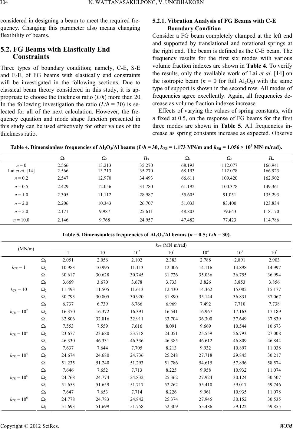

N. WATTANASAKULPONG, V. UNGBHAKORN
304
considered in designing a beam to meet the required fre-
quency. Changing this parameter also means changing
flexibility of beams.
5.2. FG Beams with Elastically End
Constraints
Three types of boundary condition; namely, C-E, S-E
and E-E, of FG beams with elastically end constraints
will be investigated in the following sections. Due to
classical beam theory considered in this study, it is ap-
propriate to choose the thickness ratio (L/h) more than 20.
In the following investigation the ratio (L/h = 30) is se-
lected for all of the next calculation. However, the fre-
quency equation and mode shape function presented in
this study can be used effectively for other values of the
thickness ratio.
5.2.1. Vibration Analysis of FG Beams with C-E
Boundar y C on d it i o n
Consider a FG beam completely clamped at the left end
and supported by translational and rotational springs at
the right end. The beam is defined as the C-E beam. The
frequency results for the first six modes with various
volume fraction indexes are shown in Table 4. To verify
the results, only the available work of Lai et al. [14] on
the isotropic beam (n = 0 for full Al2O3) with the same
type of support is shown in the second row. All modes of
frequencies agree excellently. Again, all frequencies de-
crease as volume fraction indexes increase.
Effects of varying the values of spring constants, with
n fixed at 0.5, on the response of FG beams for the first
three modes are shown in Table 5. All frequencies in-
crease as spring constants increase as expected. Observe
Table 4. Dimensionless frequencies of Al2O3/Al beams (L/h = 30, kTR = 1.173 MN/m and kRR = 1.056 × 103 MN·m/rad).
1 2 3 4 5 6
n = 0
Lai et al. [14]
2.566
2.566
13.213
13.213
35.270
35.270
68.193
68.193
112.077
112.078
166.941
166.923
n = 0.2 2.547 12.970 34.493 66.611 109.420 162.902
n = 0.5 2.429 12.056 31.780 61.192 100.378 149.361
n = 1.0 2.305 11.112 28.987 55.605 91.051 135.293
n = 2.0 2.206 10.343 26.707 51.033 83.400 123.834
n = 5.0 2.171 9.987 25.611 48.803 79.643 118.170
n = 10.0 2.146 9.768 24.957 47.482 77.423 114.786
Table 5. Dimensionless frequencies of Al2O3/Al beams (n = 0.5; L/h = 30).
kRR (MN·m/rad)
(MN/m) 1 10 102 103 104 105 106
1 2.051 2.056 2.102 2.383 2.788 2.891 2.903
2 10.983 10.995 11.113 12.006 14.116 14.898 14.997 kTR = 1
3 30.617 30.628 30.745 31.726 35.036 36.755 36.994
1 3.669 3.670 3.678 3.733 3.826 3.853 3.856
2 11.493 11.505 11.613 12.430 14.362 15.085 15.177 kTR = 10
3 30.793 30.805 30.920 31.890 35.144 36.831 37.067
1 6.737 6.739 6.766 6.969 7.492 7.710 7.738
2 16.370 16.372 16.391 16.541 16.967 17.163 17.189 kTR = 102
3 32.806 32.816 32.911 33.704 36.300 37.649 37.839
1 7.553 7.559 7.616 8.091 9.669 10.544 10.673
2 23.677 23.680 23.718 24.051 25.559 26.793 27.008 kTR = 103
3 46.330 46.331 46.336 46.385 46.612 46.809 46.844
1 7.637 7.644 7.705 8.213 9.932 10.897 11.038
2 24.674 24.680 24.736 25.248 27.718 29.845 30.217 kTR = 104
3 51.235 51.240 51.293 51.786 54.615 57.896 58.574
1 7.646 7.652 7.713 8.225 9.958 10.932 11.074
2 24.768 24.774 24.832 25.362 27.924 30.124 30.507 kTR = 105
3 51.653 51.659 51.717 52.262 55.410 59.017 59.746
1 7.647 7.653 7.714 8.226 9.961 10.935 11.078
2 24.778 24.783 24.842 25.374 27.945 30.152 30.535 kTR = 106
3 51.693 51.699 51.758 52.309 55.486 59.122 59.855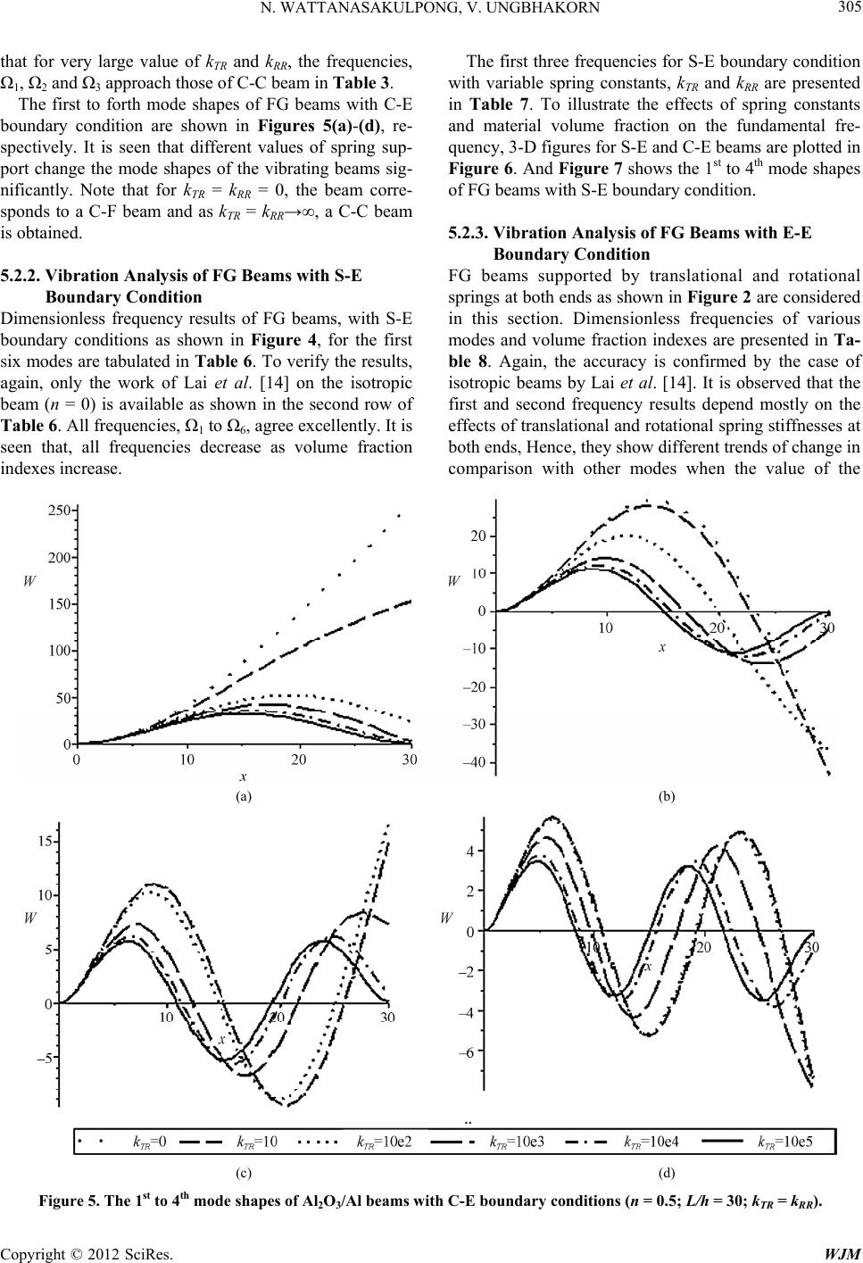

N. WATTANASAKULPONG, V. UNGBHAKORN
305
that for very large value of kTR and kRR, the frequencies,
1, 2 and 3 approach those of C-C beam in Table 3.
The first to forth mode shapes of FG beams with C-E
boundary condition are shown in Figures 5(a)-(d), re-
spectively. It is seen that different values of spring sup-
port change the mode shapes of the vibrating beams sig-
nificantly. Note that for kTR = k
RR = 0, the beam corre-
sponds to a C-F beam and as kTR = kRR, a C-C beam
is obtained.
5.2.2. Vibration Analysis of FG Beams with S-E
Boundar y C on d it i o n
Dimensionless frequency results of FG beams, with S-E
boundary conditions as shown in Figure 4, for the first
six modes are tabulated in Table 6. To verify the results,
again, only the work of Lai et al. [14] on the isotropic
beam (n = 0) is available as shown in the second row of
Table 6. All frequencies, 1 to 6, agree excellently. It is
seen that, all frequencies decrease as volume fraction
indexes increase.
The first three frequencies for S-E boundary condition
with variable spring constants, kTR and kRR are presented
in Table 7. To illustrate the effects of spring constants
and material volume fraction on the fundamental fre-
quency, 3-D figures for S-E and C-E beams are plotted in
Figure 6. And Figure 7 shows the 1st to 4th mode shapes
of FG beams with S-E boundary condition.
5.2.3. Vibration Analysis of FG Beams with E-E
Boundar y C on d it i o n
FG beams supported by translational and rotational
springs at both ends as shown in Figure 2 are considered
in this section. Dimensionless frequencies of various
modes and volume fraction indexes are presented in Ta-
ble 8. Again, the accuracy is confirmed by the case of
isotropic beams by Lai et al. [14]. It is observed that the
first and second frequency results depend mostly on the
effects of translational and rotational spring stiffnesses at
both ends, Hence, they show different trends of change in
comparison with other modes when the value of the
(a) (b)
(c) (d)
Figure 5. The 1st to 4th mode shapes of Al2O3/Al beams with C-E boundary conditions (n = 0.5; L/h = 30; kTR = kRR).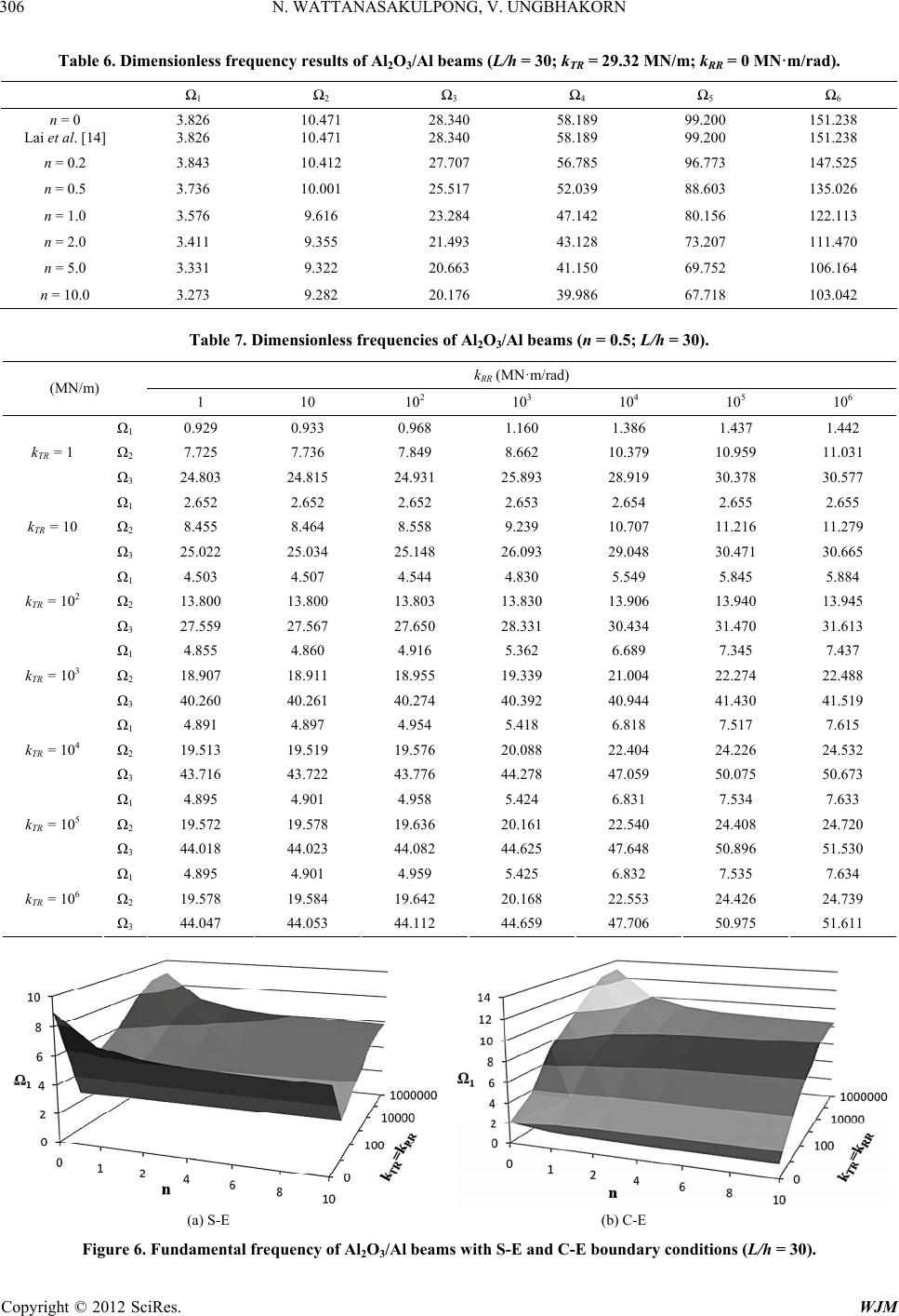

N. WATTANASAKULPONG, V. UNGBHAKORN
306
Table 6. Dimensionless frequency results of Al2O3/Al beams (L/h = 30; kTR = 29.32 MN/m; kRR = 0 MN·m/rad).
1 2 3 4 5 6
n = 0
Lai et al. [14]
3.826
3.826
10.471
10.471
28.340
28.340
58.189
58.189
99.200
99.200
151.238
151.238
n = 0.2 3.843 10.412 27.707 56.785 96.773 147.525
n = 0.5 3.736 10.001 25.517 52.039 88.603 135.026
n = 1.0 3.576 9.616 23.284 47.142 80.156 122.113
n = 2.0 3.411 9.355 21.493 43.128 73.207 111.470
n = 5.0 3.331 9.322 20.663 41.150 69.752 106.164
n = 10.0 3.273 9.282 20.176 39.986 67.718 103.042
Table 7. Dimensionless frequencies of Al2O3/Al beams (n = 0.5; L/h = 30).
kRR (MN·m/rad)
(MN/m)
1 10 102 103 104 105 106
1 0.929 0.933 0.968 1.160 1.386 1.437 1.442
2 7.725 7.736 7.849 8.662 10.379 10.959 11.031 kTR = 1
3 24.803 24.815 24.931 25.893 28.919 30.378 30.577
1 2.652 2.652 2.652 2.653 2.654 2.655 2.655
2 8.455 8.464 8.558 9.239 10.707 11.216 11.279 kTR = 10
3 25.022 25.034 25.148 26.093 29.048 30.471 30.665
1 4.503 4.507 4.544 4.830 5.549 5.845 5.884
2 13.800 13.800 13.803 13.830 13.906 13.940 13.945 kTR = 102
3 27.559 27.567 27.650 28.331 30.434 31.470 31.613
1 4.855 4.860 4.916 5.362 6.689 7.345 7.437
2 18.907 18.911 18.955 19.339 21.004 22.274 22.488 kTR = 103
3 40.260 40.261 40.274 40.392 40.944 41.430 41.519
1 4.891 4.897 4.954 5.418 6.818 7.517 7.615
2 19.513 19.519 19.576 20.088 22.404 24.226 24.532
kTR = 104
3 43.716 43.722 43.776 44.278 47.059 50.075 50.673
1 4.895 4.901 4.958 5.424 6.831 7.534 7.633
2 19.572 19.578 19.636 20.161 22.540 24.408 24.720 kTR = 105
3 44.018 44.023 44.082 44.625 47.648 50.896 51.530
1 4.895 4.901 4.959 5.425 6.832 7.535 7.634
2 19.578 19.584 19.642 20.168 22.553 24.426 24.739
kTR = 106
3 44.047 44.053 44.112 44.659 47.706 50.975 51.611
(a) S-E (b) C-E
Figure 6. Fundamental frequenc y of Al 2O3/Al beams with S-E and C-E bound ar y c onditions ( L/h = 30).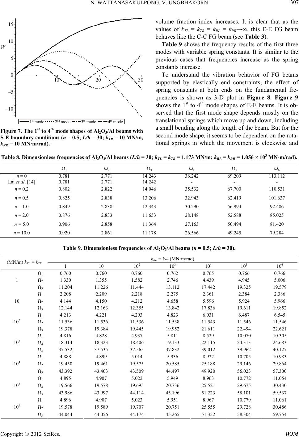

N. WATTANASAKULPONG, V. UNGBHAKORN
307
Figure 7. The 1st to 4th mode shapes of Al2O3/Al beams with
S-E boundary conditions (n = 0.5; L/h = 30; kTR = 10 M N/m ,
kRR = 10 MN·m/rad).
volume fraction index increases. It is clear that as the
values of kTL = k
TR = k RL = k RR, this E-E FG beam
behaves like the C-C FG beam (see Table 3).
Table 9 shows the frequency results of the first three
modes with variable spring constants. It is similar to the
previous cases that frequencies increase as the spring
constants increase.
To understand the vibration behavior of FG beams
supported by elastically end constraints, the effect of
spring constants at both ends on the fundamental fre-
quencies is shown as 3-D plot in Figure 8. Figure 9
shows the 1st to 4th mode shapes of E-E beams. It is ob-
served that the first mode shape depends mostly on the
translational springs which move up and down, including
a small bending along the length of the beam. But for the
second mode shape, it seems to be dependent on the rota-
tional springs in which the movement is clockwise and
Table 8. Dimensionless frequencies of Al2O3/Al beams (L/h = 30; kTL = kTR = 1.173 MN/m; kRL = kRR = 1.056 × 103 MN·m/rad).
1 2 3 4 5 6
n = 0
Lai et al. [14]
0.781
0.781
2.771
2.771
14.243
14.242
36.242
-
69.209
-
113.112
-
n = 0.2 0.802 2.822 14.046 35.532 67.700 110.531
n = 0.5 0.825 2.838 13.206 32.943 62.419 101.637
n = 1.0 0.849 2.838 12.343 30.290 56.994 92.486
n = 2.0 0.876 2.833 11.653 28.148 52.588 85.025
n = 5.0 0.906 2.858 11.364 27.163 50.494 81.420
n = 10.0 0.920 2.861 11.178 26.566 49.245 79.284
Table 9. Dimensionless frequencies of Al2O3/Al beams (n = 0.5; L/h = 30).
kRL = kRR (MN·m/rad)
(MN/m) kTL = kTR 1 10 102 103 104 105 106
1 0.760 0.760 0.760 0.762 0.765 0.766 0.766
2 1.330 1.355 1.582 2.746 4.439 4.945 5.006 1
3 11.204 11.226 11.444 13.112 17.442 19.325 19.579
1 2.208 2.209 2.218 2.275 2.361 2.384 2.386
2 4.144 4.150 4.212 4.658 5.596 5.924 5.966 10
3 12.144 12.163 12.355 13.842 17.836 19.611 19.852
1 4.213 4.221 4.293 4.823 6.031 6.487 6.545
2 11.536 11.536 11.536 11.538 11.543 11.546 11.546
102
3 19.378 19.384 19.445 19.952 21.611 22.494 22.621
1 4.816 4.828 4.937 5.811 8.529 10.070 10.305
2 18.314 18.323 18.406 19.133 22.115 24.313 24.683 103
3 37.532 37.535 37.565 37.832 39.012 39.962 40.127
1 4.888 4.899 5.014 5.936 8.922 10.705 10.983
2 19.450 19.461 19.575 20.585 25.188 29.146 29.864 104
3 43.392 43.403 43.509 44.497 49.920 56.023 57.300
1 4.895 4.907 5.022 5.949 8.963 10.772 11.054
2 19.566 19.578 19.695 20.736 25.521 29.675 30.430 105
3 43.986 43.997 44.114 45.196 51.223 58.101 59.537
1 4.896 4.907 5.023 5.951 8.967 10.779 11.061
2 19.578 19.589 19.707 20.751 25.555 29.728 30.486 106
3 44.044 44.056 44.174 45.265 51.352 58.304 59.754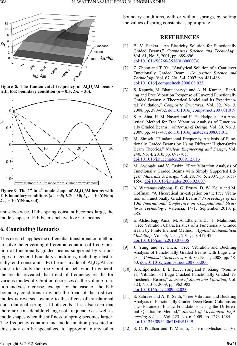

N. WATTANASAKULPONG, V. UNGBHAKORN
308
Figure 8. The fundamental frequency of Al2O3/Al beams
with E-E boundary condition (n = 0.5; L/h = 30).
Figure 9. The 1st to 4th mode shape of Al2O3/Al beams with
E-E boundary conditions (n = 0.5; L/ h = 30; kTR = 10 MN/m;
kRR = 10 MN·m/rad).
anti-clockwise. If the spring constant becomes large, the
mode shapes of E-E beams behave like C-C beams.
6. Concluding Remarks
This research applies the differential transformation method
to solve the governing differential equation of free vibra-
tion of functionally graded beams supported by various
types of general boundary conditions, including elastic-
cally end constraints. FG beams made of Al2O3/Al are
chosen to study the free vibration behavior. In general,
the results revealed that trend of frequency results for
various modes of vibration decreases as the volume frac-
tion indexes increase, except for the case of the E-E
boundary conditions in which the trend of the first two
modes is reversed owning to the effects of translational
and rotational springs at both ends. It is also seen that
there are considerable changes of frequencies as well as
mode shapes when the stiffness of spring becomes larger.
The frequency equation and mode function presented in
this study can be specialized to approximate any other
boundary conditions, with or without springs, by setting
the values of spring constants as appropriate.
REFERENCES
[1] B. V. Sankar, “An Elasticity Solution for Functionally
Graded Beams,” Composites Science and Technology,
Vol. 61, No. 5, 2001, pp. 689-696.
doi:10.1016/S0266-3538(01)00007-0
[2] Z. Zhong and T. Yu, “Analytical Solution of a Cantilever
Functionally Graded Beam,” Composites Science and
Technology, Vol. 67, No. 3-4, 2007, pp. 481-488.
doi:10.1016/j.compscitech.2006.08.023
[3] S. Kapuria, M. Bhattacharyya and A. N. Kumar, “Bend-
ing and Free Vibration Response of Layered Functionally
Graded Beams: A Theoretical Model and Its Experimen-
tal Validation,” Composite Structures, Vol. 82, No. 3,
2008, pp. 390-402. doi:10.1016/j.compstruct.2007.01.019
[4] S. A. Sina, H. M. Navazi and H. Haddadpour, “An Ana-
lytical Method for Free Vibration Analysis of Function-
ally Graded Beams,” Materials & Design, Vol. 30, No. 3,
2009, pp. 741-747. doi:10.1016/j.matdes.2008.05.015
[5] M. Simsek, “Fundamental Frequency Analysis of Func-
tionally Graded Beams by Using Different Higher-Order
Beam Theories,” Nuclear Engineering and Design, Vol.
240, No. 4, 2010, pp. 697-705.
doi:10.1016/j.nucengdes.2009.12.013
[6] M. Aydogdu and V. Taskin, “Free Vibration Analysis of
Functionally Graded Beams with Simply Supported Ed-
ges,” Materials & Design, Vol. 28, No. 5, 2007, pp. 1651-
1656. doi:10.1016/j.matdes.2006.02.007
[7] N. Wattanasakulpong, B. G. Prusty, D. W. Kelly and M.
Hoffman, “A Theoretical Investigation on the Free Vibra-
tion of Functionally Graded Beams,” Proceedings of the
10th International Conference on Computational Struc-
tures Technology, Valencia, 14-17 September 2010, p.
285.
[8] E. Alshorbagy Amal, M. A. Eltaher and F. F. Mahmoud,
“Free Vibration Characteristics of a Functionally Graded
Beam by Finite Element Method,” Applied Mathematical
Modelling, Vol. 35, No. 1, 2011, pp. 412-425.
doi:10.1016/j.apm.2010.07.006
[9] J. Yang and Y. Chen, “Free Vibration and Buckling
Analysis of Functionally Graded Beams with Edge Cra-
cks,” Composite Structures, Vol. 83, No. 1, 2008, pp. 48-
60. doi:10.1016/j.compstruct.2007.03.006
[10] S. Kitipornchai, L. L. Ke, J. Yang and Y. Xiang, “Nonlin-
ear Vibration of Edge Cracked Functionally Graded Ti-
moshenko Beams,” Journal of Sound and Vibration, Vol.
324, No. 3-5, 2009, pp. 962-982.
doi:10.1016/j.jsv.2009.02.023
[11] S. Sahraee and A. R. Saidi, “Free Vibration and Buckling
Analysis of Functionally Graded Deep Beam-Columns on
Two-Parameter Elastic Foundations Using the Differen-
tial Quadrature Method,” Journal of Mechanical Engi-
neering Science, Vol. 223, No. 6, 2009, pp. 1273-1284.
doi:10.1243/09544062JMES1349
[12] S. C. Pradhan and T. Murmu, “Thermo-Mechanical Vi-

N. WATTANASAKULPONG, V. UNGBHAKORN
309
bration of FGM Sandwich Beam under Variable Elastic
Foundations Using Differential Quadrature Method,” Jour-
nal of Sound and Vibration, Vol. 321, No. 1-2, 2009, pp.
342-362. doi:10.1016/j.jsv.2008.09.018
[13] J. C. Hsu, H. Y. Lai and C. K. Chen, “Free Vibration of
Non-Uniform Euler-Bernoulli Beams with General Elas-
tically End Constraints Using Adomain Modified Decom-
position Method,” Journal of Sound and Vibration, Vol.
318, No. 4-5, 2008, pp. 965-981.
[14] H. Y. Lai, J. C. Hsu and C. K. Chen, “An Innovative Ei-
genvalue Problem Solver for Free Vibration of Euler-
Bernoulli Beam by Using the Adomain Decomposition
Method,” Computers & Mathematics with Applications,
Vol. 56, No. 12, 2008, pp. 3204-3220.
doi:10.1016/j.camwa.2008.07.029
[15] Y. Liu and C. S. Gurram, “The Use of He’s Variational
Iteration Method for Obtaining the Free Vibration of an
Euler-Bernoulli Beam,” Mathematical and Computer Mo-
delling, Vol. 50, No. 11-12, 2009, pp. 1545-1552.
doi:10.1016/j.mcm.2009.09.005
[16] Q. Mao and S. Pietrzko, “Free Vibration Analysis of
Stepped Beams by Using Adomian Decomposition Me-
thod,” Applied Mathematics and Computation, Vol. 217,
No. 7, 2010, pp. 3429-3441.
doi:10.1016/j.amc.2010.09.010
[17] J. K. Zhou, “Differential Transformation and Its Applica-
tion for Electrical Circuits,” Huazhong University Press,
Wuhan, 1986.
[18] M. Malik and H. H. Dang, “Vibration Analysis of Con-
tinuous Systems by Differential Transformation,” Applied
Mathematics and Computation, Vol. 96, No. 1, 1998, pp.
17-26. doi:10.1016/S0096-3003(97)10076-5
[19] M. O. Kaya and O. O. Ozgumus, “Flexural-Torsional-Cou-
pled Vibration Analysis of Axially Loaded Closed-Sec-
tion Composite Timoshenko Beam by Using DTM,” Jour-
nal of Sound and Vibration, Vol. 306, No. 3-5, 2007, pp.
495-506.
[20] O. O. Ozgumus and M. O. Kaya, “Flapwise Bending Vi-
bration Analysis of Double Tapered Rotating Euler-Bur-
noulli Beam by Using the Differential Transform Me-
thod,” Meccanica, Vol. 41, No. 6, 2006, pp. 661-670.
doi:10.1007/s11012-006-9012-z
[21] O. O. Ozgumus and M. O. Kaya, “Vibration Analysis of a
Rotating Tapered Timoshenko Beam Using DTM,” Mec-
canica, Vol. 45, No. 1, 2010, pp. 33-42.
doi:10.1007/s11012-009-9221-3
[22] S. C. Pradhan and G. K. Reddy, “Buckling Analysis of
Single Walled Carbon Nanotube on Winkler Foundation
Using Nonlocal Elasticity Theory and DTM,” Computa-
tional Materials Science, Vol. 50, No. 3, 2011, pp. 1052-
1056. doi:10.1016/j.commatsci.2010.11.001
[23] F. Delale and F. Erdogan, “The Crack Problem for a Non-
Homogeneous Plane,” Journal of Applied Mechanics, Vol.
50, No. 3, 1983, pp. 609-614. doi:10.1115/1.3167098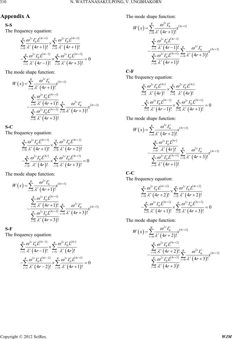

N. WATTANASAKULPONG, V. UNGBHAKORN
310
Appendix A
S-S
The frequency equation:








4141 22
00
00
41 43
22
00
10
41! 41!
0
41! 43!
rr rr rr
RR
rr
rr
rr
rrrr
RR
rr
rr
IL IL
rr
IL IL
rr










 



The mode shape function:
 







2
41
0
0
41
2
0
2
043
0
43
20
0
0
41!
41!
43!
43!
rr
Rr
r
r
r
rr
R
rrr
R
rr
r
r
rr
Rr
r
r
I
Wx x
r
IL
rIx
r
IL
r





















S-C
The frequency equation:








41 42
22
00
00
443
22
00
00
41!42!
0
4!4 3!
rr
rr rr
RR
rr
rr
rr
rr rr
RR
rr
rr
IL IL
rr
IL IL
rr










 



The mode shape function:
 







2
41
0
0
41
2
0
2
043
0
43
20
0
0
41!
41!
43!
43!
rr
Rr
r
r
r
rr
R
rrr
R
rr
r r
rr
Rr
r
r
I
Wx x
r
IL
rIx
r
IL
r





















S-F
The frequency equation:








41 4
22
00
10
42 41
22
00
10
41! 4!
0
42! 41!
rr
rrrr
RR
rr
rr
rr
rrrr
RR
rr
rr
ILIL
rr
ILIL
rr










 



The mode shape function:
 







2
41
0
0
41 2
0
2
143
0
41
20
0
0
41!
41!
43!
41!
rr
Rr
r
r
r rr
R
rrr
R
rr
r r
rr
Rr
r
r
I
Wx x
r
IL
rIx
r
IL
r





















C-F
The frequency equation:








44
22
00
00
41 41
22
00
10
4! 4!
0
41! 41!
rr
rrrr
RR
rr
rr
rr
rrrr
RR
rr
rr
IL IL
rr
IL IL
rr













The mode shape function:
 







2
42
0
0
4 2
0
2
043
0
41
20
0
0
42!
4!
43!
41!
rr
Rr
r
r
r rr
R
rrr
R
rr
r
r
rr
Rr
r
r
I
Wx x
r
IL
rIx
r
IL
r



















C-C
The frequency equation:








42 42 22
00
00
41 43
22
00
00
42! 42!
0
41!43!
rr rrrr
RR
rr
rr
rr
rr rr
RR
rr
rr
IL IL
rr
IL IL
rr















The mode shape function:
 







2
42
0
0
42
2
0
2
043
0
43
20
0
0
42!
42!
43!
43!
rr
Rr
r
r
r
rr
R
rrr
R
rr
r
r
rr
Rr
r
r
I
Wx x
r
IL
rIx
r
IL
r




















