 American Journal of Computational Mathematics, 2012, 2, 302-311 http://dx.doi.org/10.4236/ajcm.2012.24041 Published Online December 2012 (http://www.SciRP.org/journal/ajcm) Super-Resolution with Multiselective Contourlets Mohamed El Aallaoui1, Abdelwahad Gourch2 1Laboratory of Mathematical Engineering (LINMA), Department of Mathematics and Computer Science, Faculty of Sciences, Eljadida, Morocco 2Faculté des Sciences Juridiques, Économiques et Sociales de Ain Sebaâ, Casablanca, Morocco Email: m_elaallaoui@yahoo.fr, agourch2002@yahoo.fr Received July 18, 2012; revised September 19, 2012; accepted October 10, 2012 ABSTRACT We introduce a new approach to image super-resolution. The idea is to use a simple wavelet-based linear interpolation scheme as our initial estimate of high-resolution image; and to intensify geometric structure in initial estimation with an iterative projection process based on hard-thresholding scheme in a new angular multiselectivity domain. This new do- main is defined by combining of laplacian pyramid and angular multiselectivity decomposition, the result is multiselec- tive contourlets which can capture and restore adaptively and slightly better geometric structure of image. The experi- mental results demonstrate the effectiveness of the proposed approach. Keywords: Super-Resolution; Laplacian Pyramid; Angular Multiselectivity; Multiselective Contourlets; Anti-Aliasing Filer; Sparsity Constraint; Iterative Projection 1. Introduction In most digital imaging applications, high-resolution im- ages or videos are usually desired for later image proc- essing and analysis. The desire for high resolution stems from two principal application areas: improvement of pictorial information for human interpretation; and help- ing representation for automatic machine perception [1,2]. Image resolution describes the details contained in an image, the higher the resolution, the more image details [1,3]. Super-resolution is techniques that construct high- resolution images from several observed low-resolution images, thereby increasing the high-frequency compo- nents and removing the degradations caused by the im- aging process of the low-resolution camera. The basic idea behind super-resolution is to combine the non-re- dundant information contained in multiple low-resolution frames to generate a high-resolution image. The super- resolution (SR) reconstruction of a digital image can be classified in many different ways: SR in spatial domain [4,5], SR in the Frequency Domain [6,7], Statistical Ap- proaches [8,9], and Interpolation-Restoration [1,10]. In this last context, can be distinguished two categories, linear and nonlinear interpolation methods. Linear interpolation methods, such as bilinear, bicubic and cubic spline [11,12], edge-sensitive filter [13], blur- ring and ringing effects because they do not utilize any information relevant to geometric structure of image [14,15]. Nonlinear interpolation methods incorporate more adaptive image models and priori knowledge which often improve linear interpolators. Many approaches have been designed for addressing this task in recent years. We may cite for instance, Soft-decision Adaptive Interpolation (SAI) [16], Sparse Mixing Estimators (SME) [17], Iterative Projection [18], ··· The SAI approach has been improved by Zhang and Wu, by using an interpolator adapted to local covariance image based on autoregressive image models optimized over image blocks. This approach can be more accurate, it is much more demanding in computation and memory resources. The SME approach proposed by Mallat and Yu, computes a high-resolution estimator by mixing adaptively a family of linear estimators corresponding to different priors. Sparse mixing weights are calculated over blocks of coefficients in a frame providing a sparse signal representation. Mueller and Lu have proposed an iterative interpolation method based on the wavelet and contourlet transforms [19,20]. In this approach, the con- tourlet transform improves the visual quality of resulting images, by intensification of the geometric structure on the wavelet linear interpolation. This geometric structure is well represented by contourlets with variable angular selectivity [21]. However, the contoulets represent the image geometry with the same angular selectivity [19,20]. In order to overcome this limitation of representation of geometric structure in this iterative approach, we have increased the sensitivity of angular selectivity of con- tourlets. Our idea is based on a simple wavelet-based linear interpolation scheme as our initial estimate; and an iterative projection process based on hard-thresholding C opyright © 2012 SciRes. AJCM  M. EL AALLAOUI, A. GOURCH 303 scheme in a new angular multiselectivity domain. This new domain is defined by combining of laplacian pyra- mid and an angular multiselectivity decomposition. The result is new multiselective contourlets, which can rep- resent the different structures of the image geometry. The paper is organized as follows. In Sections 2 and 3, we discuss the new multiselective contourlets, and we will show how these multiselective contourlets can pro- vide a new degree of freedom to describe adaptively the different structures of the image geometry. Our multise- lective contourlets algorithm for image super-resolution is described in the Section 4. We report the results of our experiments in Section 5 and conclude the paper in Sec- tion 6. 2. Laplacian Pyramid The Laplacian Pyramid was first proposed in [22] as a new technique for compression image. To achieve high compression, it removes image correlation by com- bining predictive and transform coding techniques. LP In the Laplacian Pyramid decomposition at each level the original image happens in a high-pass and a low-pass filters, the resulting is a downsampled low-pass version of the original image, and of difference between the original image and the prediction. Under certain regularity conditions, the low-pass filter in the iterated uniquely defines a unique scaling LP function that satisfies the following two- scale eq 22 tL uation [23,24] 222 n tgt .n (1) Let 2 , 2 2,, 2 j j jn j tn tj . n (2) Then the family is an orthonormal basis fo 2 ,jn n r an approximation subspace V at the scale 2 . Furthermore, j V provides a sequence of multire- solution neste , d subspaces 2101 2 VVVV V where V is associated with 22 a uniform grid of intervals j at characterizes image approximation at scale th 2 . Th nec e difference images in the LP contain the details essary to increase the resolutioetween two conse- cutive approximation subspaces. Therefore, the diffe- rence images live in a subspace n b W that is the orthogonal complement of V in 1 V, or 1. j j (3) The can be considered as an oversampled filter ba here VVW LP nk w each polyphase component of the difference signal comes from a separate filter bank channel like the coarse signal [25]. Let ,0 3 i zi be the synthesis filters for these polypha. Note that these synthesis filters are high-pass filters. As for wavelets, we associate with each of these filters a continuous function se components it where 2 22 i n tf .n it ): let (4) osition 2.1 ([25]Prop 2 , 2 2,, 2 j iji jn j n tj .n (5) , for scale t Then2 , 2 ,03, i jn in is a tight frame for W. Since W is generated by four kernel functions (similar to multi-wavelets), in general it is not a shift- invariant subspace. Nevertheless, we can simulate a shift- invariant subspace by denoting i t ,2, ,0 3. i jn k jnti (6) are the coset representatives for downsam T T (7) this notation, the family associated where With to a i k i p- ling by 2n each dimension T 0,0 ,k 01 T 23 1,0, 0,1,1,1 . k kk 2 ,jn n 11 n uniform grid of intervals 22 j on 2 pro- vides a tight frame for W n theamily [25]. The f 2 ,jn n suffices the follog equality: win 2 22 ,,. nj j n ffW (8) elective Contourlets elective contourlets eriodic function 3. Multis In this section we propose the multis defined by combining of laplacian pyramid and an angu- lar multiselectivity decomposition, and we will show how these new contourlets can provide a new degree of freedom to describe adaptively the different structures of the image geometry. We consider 2π-p defined by ,0,2; 1,2, π; π,π,π2; 0, π2,2π. (9) Copyright © 2012 SciRes. AJCM  M. EL AALLAOUI, A. GOURCH 304 0,π and the function where is defined in 1,1 and satisfies the followingerty: prop 221.tt For and (10) * Lπ 2 , we create 2l different - periodic functions 2π ,lm indexed by for any de 02 l m 0,lLfined by: , 0,0 1, (11) 1,2 , 21π, l m ) 2 lm lm (12 1,2 1lm , π. 2 lm l By the laplacian pyramidc wavelets 21πm (13) , n bspace defined in the previous section and for each su W r transf , we construct a new contourlets whose Fouriorms are: e ,,,, , ˆˆ, jnlmjn lm kk where (14) arg k. osition 3.Prop1 for any 1, ,lL ,0l 1 1 11 1 ,0,2; π 1,2 ,; 2 ππ 2,,2; 22 π 0,2, 2π. 2 l l ll l π (15) and 0, ,21 l m ,,,, , ,,0 ˆˆ 2π ˆ. 2 jnlmjn lm jn ll m kk k (16) Proof According to the expression (9) of the function , π 2 π 0,0 ,; 2 π ππ 2,,2; 22 ll ππ 1, 2 ,π; 22 π π+ππ 2,π,π2; 22 π 0, π2,2π. 2 l l l ll l ll l one have for any 1, ,lL: (17) π π2 π 1,0 ,; 2 π ππ 2,,2; 22 ππ 0,2 ,π; 22 π πππ 2,π,π2; 22 π 1, π2,2π. 2 l l l ll ll l ll l (18) We shall now prove that for any L 1, ,l 1 ,0 1 11 1 ,0,2; π 1,2 ,; 2 π ππ 2,, 22 π 0,2, 2π. 2 l ll ll l 2; (19) Let’s prove this by induction: Since 1,0 0,0ππ , the function 1,0 Copyright © 2012 SciRes. AJCM  M. EL AALLAOUI, A. GOURCH 305 expressed as (19). Now assume that for a fixed , the function l ,0l n h expressed as (19). The inclusiothis inductioypothesis and Equation (18) in the ex- pression (12) gives: n of 1,0 ,0,2; π 1,2 ,; 2 π ππ 2,,2; 2 l ll ll (20) e expressions (17) and (19) in Equation (13) shows that: for any 2 π 0, 2, 2π. 2l This last result completes the proof of the induction. The insertion of th 1, ,lL 1 1 11 ,1 12 2ππ 2,, 2; l 22 22 ll 2 π 0,0,; 2 π ππ 2,,2 22 ππ 1,2 ,; 22 π π 0,2 ,2π. 2 l l ll lll l ; (21) Therefore, for any 1, ,lL ,1 ,0 1 π. 2 ll l (22) We shall now prove that, for any L (23) Let’s prove this by induction: Now assume that for a fixed (24) with 1, ,l ,,0, 0,1,, 21. l lmllm m l: ,,0, 0,1,, 21 l lmllm m , 2π. 2 lm l The inclusion of th m e induction hypothesis and Equ- ation (22) in the expressions (12) and (13) gives: 1,01,2 ll m 1,2, ,0 ,, 1,2 21 π2 π π2 π2 , lm lml llm lm l lm l m ,0 1,2 ll m π π 1,21, ,0 1,21,2 1,11,21,01,2 1 21π 2 π 2 . lm lml llm lm l llmllm m The proposition shows that for each level of con- struction l, the functions ,0 ,, 2 π ll m lm l ,lm are continuous with co- pact support of size m 2π2 2l . So the aperture of the cone in frequency space supporting of ,,, ˆ nlm is equal to 2π2 2l . Therefore, the contourlets ,,, nlm are directional [26,27], and the angular selectivity of these new contourlets is proportional to . Keeping that in mind, we will call the new cont 2l ourlets ,,, nlm the mu tiselective contourlets, and the paramangular selectivity level. The central result is that for each selectivity level the multiselective contourlets generate a tight frame each subspace l- eter l the l, for W. Theorem 3.1 for any 0, ,lL the family 2 ,,,:,0,1,1 l jnlm nm ,2 is a tight frame for W. Proof To prove that the family 2,0,1,,21 l m ,, ,: jnlm n is a tighte for fram Wes to evaluate the equality: , it suffic 2 21 2 ,,, 0 ,. l2 nlm j m n ffW (25) Define the quantities 2 21 2 ,,,, 0 , l jnjlm m n Ef f (26) and ,,, ,, ˆˆ jnlmjlm kk ,, 2. j jlm n k (27) Let us prove first that Copyright © 2012 SciRes. AJCM  M. EL AALLAOUI, A. GOURCH 306 Ef 21 2ˆ 4π l f kk ˆ2d. j fn k k (28) 2 2,, , 0jnlm m n We have ddff xxx 22 2 2 22 2 ,,,, ,,, ,,, ,, ,, i2 ,, i2 ,, ,, 2d 2d ˆ ˆ ed d ˆˆ ˆˆ ed j j jnjlm jnlm jnlm j jlm j jlm njlm njlm jlm f fn fn f ff k kk x xx xxx xxx kkk k kkkkkk Using the Poisson formula (29) We obtain . We shall now prove that (30) According to the property (10), we verify that (31) 2 i2 ,, ˆ ˆ e jnjlmf kkk 2 d. 22 i2 2 e4π2. jnj nn n kk kk 2 2 21 2 ,,, 0 ˆˆ 4π2d l j jnlm m n Ef ff n kk kk 21 ,,, 0 ˆˆ 2. l j jnlmj j m n kkk 22 π1. Hence, for any 0, ,lL 1 21 ,1,,0, 1, ˆˆ 2 l jl mj lm kk 1 0 21 l 1 21 ,,, ,,2 ,,2 0 ,,2 1,,2 1 21 2 , 0 2 , 1,, 1,, 0 ˆ2 ˆ2 2 ˆˆ2π l l jnlm m j jl mjl m m j jl mjl m jml m j jl mjl mml m n n n n k kk kk k kk ,1,, 1, ˆˆ jl mjl m k 1 22 , 21 , 1,, 1,,,1, 00 π ˆˆ2, l ml j jl mjl mjnl m mm n kk k with 1 , 21 l ml jn ,1 21π. 2 ml l m Therefore, The equalities (8), (26), (28) and (30) imply that 21 ,,, ,,0,0 0 ˆˆ 2 l j jnlmjnj j m n kkkk 2 2 2 22 2 22 2 2 21 2 ,,, 0 2 i2 i2 ,, 22 ,, ˆˆ ˆˆ 4π22 ˆˆ ˆˆ ede dd . l jj jnlm m n jj jj jj n nn jj n jn jn n jn d d f nf f n ff ff ff kk kkkk k kkkkkk xxxx xx fore, for each selectivity level , any function n There l W is represented as: 2 2 1 ,,, ,,, 0 . l njlm jnlm m n ff xx (32) Since J 00 Jj VV W , any jj0 V is repre- sented as: 2 2 20 ,, 1 ,,,,,, 0 , Jn Jn n Jl jnlm jnlm jjm n f xx x (33) with ,, , Jn Jn (34) ,,,,,, , jnlm jnlm (35) and t orthogonal s im t for each selectivity lethe the he decompositions of 22 L into mutual ubspaces: 22 , Jj jJ LVW (36) ply thavel l, family 2 , :,,0,1,,2 l mnjJm ,, , , 1 Jn jnl is a tight frame for 22 L, on which any function 22 fL is represented as: 2 2 2 ,, 1 ,,, ,,, 0 Jn Jn n l jnlmjnlm jJm n f xx x (37) Copyright © 2012 SciRes. AJCM 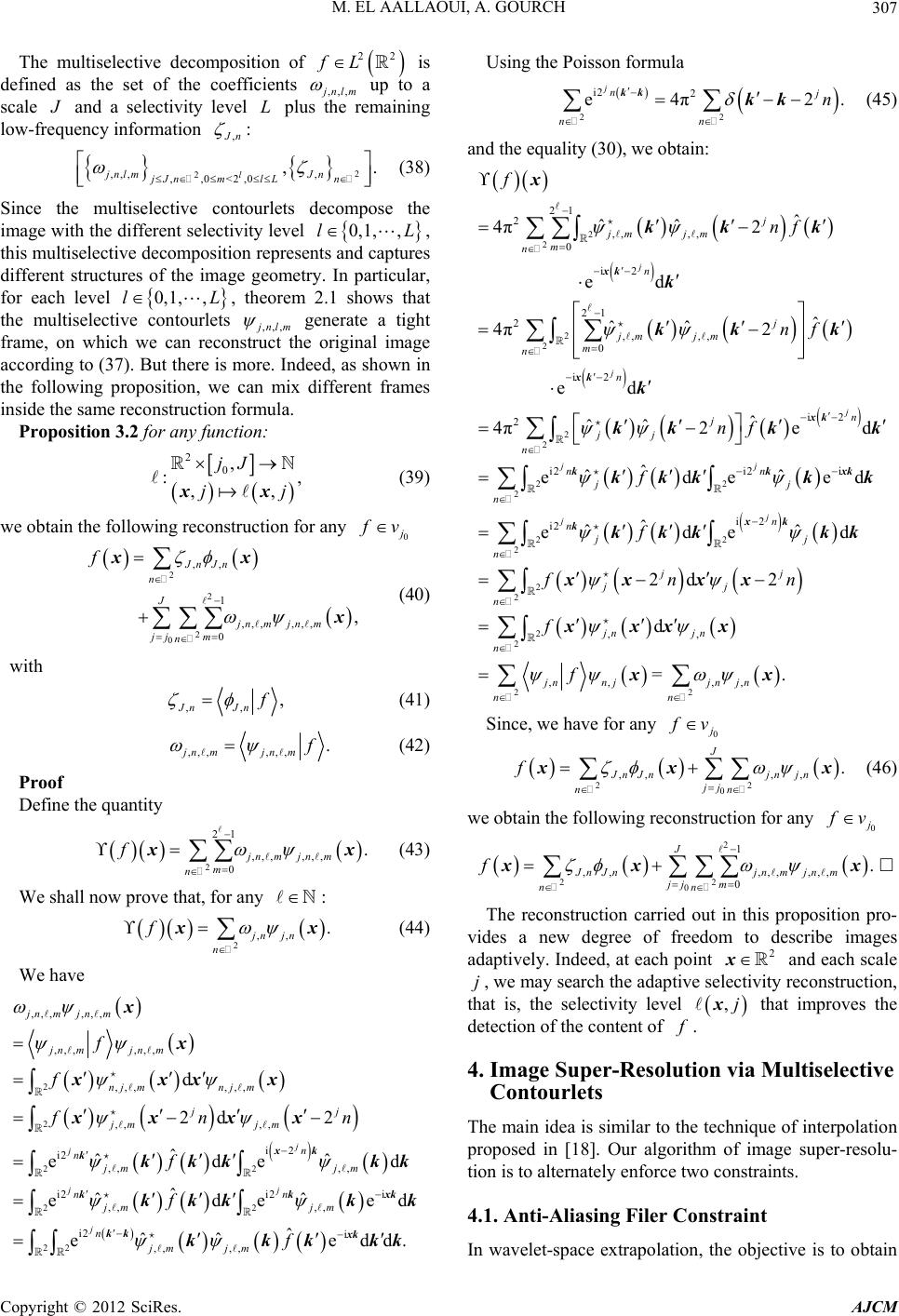 M. EL AALLAOUI, A. GOURCH 307 sition of 22 fL is ficients The multiselective decompo defined as the set of the coef,,, nlm up to a scale req and a selectivity level low-fuency information L plus the remaining , n : ,,,jnlm jJ (38) 2 2, ,,0<2,0 ,. lJn n nmlL Since the multiselective contourlets de image with the different selectivity level this multiselective decomposition represen for each level, theorem the multiselec compose the 0,1, ,, lL ts and captures , 2.1 s different structures of the image geometry. In particular 0,1, ,lL tive contourlets hows that ,,, nlm whi ut there is more. Indeed, as shown in the following proposition, we can mix different frames inside the same reconstruction formula. Proposition 3.2 for any function: generate a tight iginal imageframe, on e can reconstruct the or ch w according to (37). B 2 0, :, ,, jJ jj xx (39) any we obtain the following reconstruction for0 v 2,,Jn Jn n f xx 2 2 0 1 ,,,,,, 0 , J jn mjn m jjm n x (40) with ,, , Jn Jn (41) ,,,,,, . jn mjn m We shall now prove that, for any (42) Proof Define the quantity 21 ,,,,. jn mj f xx (43) 20m n ,,n m : 2,,jn jn n f x .x (44) We have 2ˆd jn kkk 2 22 22 ,,,,,, ,,, ,,, ,,,,,, ,, ,, i i2 ,, ,, i2 i2 ,, ,, d 2d 2 ˆ ˆ ede ˆ ˆˆ ede j jj jn mjnm jn mjn m nj mnj m jj jm jm njm jm nn jm jm f f nn f f x k kk x x xxxx xxxx kkk kkk i ,, ˆ ˆe dd. jnjmf kk xk kk kkk Using the Poisson formula (45) and the equality (30), we obtain: i e xk kdk 2f i2 22 ,, ˆ e jm i2 2 e4π2. jnjn kk kk 22 nn 2 2 2 2 2 2 2 2 1 2 ,, ,, 0 i2 21 2 ,, ,, 0 i2 i2 2 i2 ˆ ˆˆ 4π2 ed ˆ ˆˆ 4π2 ed ˆ ˆˆ 4π2e ˆ e j j j j j jmjm m n n j jmjm m n n n j jj n nj f nf nf nf 2 d n xk xk xk k x kk k k kkk k kkk k 2 22 2 2 2 2d j n fn xxx 2 2 22 i2 i i2 ,, ,, ,, ˆˆ de ed ˆˆ eded 2 d =. j j nj n jj n jj j jn jn n jnnjjn jn nn f f n f f kxk xk kkkk k kkk k x xxxx xx Since, we have for any i2 ˆ jnkk 0 v x (46) we obtain the following reconstruction for any 22 0 ,,, ,. J Jn Jnjnjn jj nn f xx 0 v x The reconstruction carried out in this proposition pro- vides a new degree of freedom to describe images adaptively. Indeed, at each point and each scale we may search the adaptive ity reconstruction, at is, the selectivity level at improves the detection of the content of 2 22 0 1 ,,,,, ,,, 0 . J JnJnjnmjnm jjm nn f xx 2 x selectiv ,jx th j, th . 4. Image Super-Resolution via Multiselective Contourlets The main idea is similar to the technique of interpolatio proposed in [18]. Our algorithm of image super-resolu- tioe two constraints. 4.1. Anti-Aliasing Filer Constraint In wavelet-space extrapolation, the objective is to obtain n n is to alternately enforc Copyright © 2012 SciRes. AJCM  M. EL AALLAOUI, A. GOURCH 308 an estimation 0 ˆ of high-resolution image x from low- resolution image (refer to Figure 1). In this case we impose anti-al filer constraint, that is the given low-resolution ie is the downsampled output of the lo iasi m ng ag w-pass anti-aliasing filter in a wavelet transform. As a simple way to get an estimate 0 ˆ of the high resolution image, we can take the inverse vet transform by keping wa el e as the low-pass band and zeropadding all high-pass subbands. Consequenr any given image y, we can calculate the best approx2 L norm) to y, subject to anti-aliasing filer con tly, fo imation (in s, through traint orthogonal projection. Let and 1 represent the forward and inverse wavelet transforms, respectively; ote P as the diden onal 1s and 0s sforms, culated by (47) e n de multiselective contourlet coefficients. agprojection matrix of that keeps the low-pass wavelet coefficients and zeros out the high frequency subband coefficients, and let PIP . If we use orthonormal wavelet tran then the projection of any image y can be cal 1 ˆˆ 0,yF PFyPFx where 0 ˆ x is thestimation of the high-resolution image obtained as in Figure 1. 4.2. Sparsity Constraint The second constraint is based on a model for natural images. Since the multiselective contourlets described in Section 3, generate a multiselective geometric represen- tation well-suited to preserve contours and edges and geometric structure of image, we assume that the un- known high-resolution image should be sparse in the multiselective contourlets domain. For the sake of sim- plicity, we choose to use a direct hard-thresholding scheme i our proposed algorithm. Intuitively, we view our estimate to the high-resolution image as a noisy ver- sion of the true image. Enforcing our sparsity constraint works tonoise the estimation of the interpolated signal while retaining the important coefficients near edges. we enforce this constraint through a hard-thresholding of the We suppose that the estimation ˆ of the high- resolution is a multiresolution approximation of the real image f at the resolution. Hence 0 20 ˆ V, and the om of multiselective contourlets decposition ˆ is ficients defined as the set of the coef ,,,,,, ˆ jnlmjnlm up to a scale 0J and a sele- Figure 1. The anti-aliasing filer constraint. ctivity level 0L, plus the remaining low-frequency information ,, ˆ Jn Jn : 2 2 ,,, , 0,,02,0 ˆ,. l jnlmJn n jJnm lL x (48) Denote T as the diagonal matrix that, given some threshold value T, zeros out insignificat coefficients in the coefficient vector whose absolute values are smaller than T; and as the adaptive selectivity reconstruction given by proposition (3.2), n ,, ˆJn Jn x 2 2,,, ,,, 10 . n jn mjnm jm n 21J t (49) tt we choice the adaptive selectivity level by mini- mizing the distortion introduced by thre in fixed selectivity procedure: ,jt sholding 22 L nn with ,,0,0,,,0 0, ,argminjn jnl l ttt,j (50) 21 ,,,0,,, ,,, 0 . l jnlTjnlm jnlm m tt (51) Denote the denoised high-resolution image. The sparseness constraint by hard-thresholding can be written as ˆ. T x (52) 4.3. Multiselective Contourlets Algorithm for Image Super-Resolution We show in Figure 2 the block diagram of the proposed r high- thm by taking multiselective contourlets algorithm foresolution image reconstruction, which can be summarized as fol- lows: 1) We start our algori 0 ˆ , obtained by the simple wavelet interpolation shown in Figure the initial estimate of the high-resolution image. 2) We then attempt to improve the quality of inter- on, particularly in regions containing edges and contours, by iteratively enforcing the observation con- straint as well as the sparseness constraint. Let 1, as polati ˆk re- present the estimate at the kth step. By comb and (52), the ining (47) new estimate 1 ˆk can then be obtained by 1 10 ˆˆˆ. k kTk FPF xPFx (53) 3) Following the same principle o based image recovery algorithm proposed in [28], we all amo f the sparseness- gradually decrease the threshold value k T by a sm unt in each iteration, i.e., 1kk TT rcumng t venti . This has been shn to be effective in cihe non- ow Copyright © 2012 SciRes. AJCM  M. EL AALLAOUI, A. GOURCH 309 Figure 2. The block diagram of the proposed algorithm for image super-resolution. convexity of the sparseness constraint. We compare the high-resolution images obtained by the proposed method with those obtained by wavelet linear [28], interpolation bicubic [29], contourlet transform [18], soft-decision adaptive interpolation (SAI) [16], and sparse mixing estimators (SME) [17]. In the experiments, we use five scales J = 5, and five selectivity level 4) Return to step 2 and keep iterating, until the gene- rated images converge or a predetermined maximum iteration number has been reached. 5. Numerical Experiments 5L d we for multiselective contourlets decomposition, an choose and is decreased by 010T 0.2 erations 512 in each . We use 2, in- iteratia maximum of 10 it severalrd test images of size cluding Lenna, Boat, Gauss disc, Peppers, Straws, and gular regions. Peppers is mainly composed of regular Mandril is rich in fin ms, we first down- sampled each image by a factor of 2 and then inter- on, with standa51 Mandril (Figure 3). Gauss disc image includes regular regions, Lenna and Boat include both fine details and re regions separated from sharp contours. e details. Straws image contains directional patterns that are superposed in various directions. To show the true power of the interpolation algorith polated the result back to its original size. The performance measure used was the Peak Signal to Noise Ratio (PSNR), A good high-resolution method must maximize the PSNR. Table 1 gives the PSNRs generated by all methods for the images in Figure 3. Figures 4 and 5 compare the high-resolution image obtained by different methods. Bicubic interpolations produce some blur and jaggy artifacts in the zoomed images, but the image quality is lower than with SME and SAI methods, as shown by the PSNRs. The Con- tourlet method yields almost the same PSNR as a bicubic interpolation but often provides better image quality. It is able to restore the geometrical structures (see Lenna’s hat and gauss disc zoom) when the underlying contourlet Figure 3. Images used in the numerical experiments. Figure 4. The zoom-in comparison of the Lenna and Gauss disc images. From left to right: high-resolution image, low- resolution image (shown at the same scale by enlarging the pixel size), wavelet linear, bicubic interpolation, contourlet, SME, SAI, and proposed method. vectors are accurately estimated. However, when the approximating contourlet vectors are not estimated correctly, it produces directional artifact patterns, be- cause the contoulets represent the image geometry with the same angular selectivity. Contrariwise in our pro- posed method, the angular selectivity can be adapted locally to the content of the image, which improves its gain in PSNR and its regularity of object boundaries of geometrical structures in the generated images, as shown in Boat and Peppers zooms. Copyright © 2012 SciRes. AJCM  M. EL AALLAOUI, A. GOURCH Copyright © 2012 SciRes. AJCM 310 Table 1. The performance of the proposed method relative to oth of Figure 3. From left to right: wavelet linear [28], interpolat estimators (SME) [17], and soft-decision adaptive interpolation (S Image Wavelet lin Bicubic Contour Proposed er methods. PSNRS (in decibels) are computed over images ion bicubic [29], contourlet transform [18], sparse mixing AI) [16]. let SME SAI Lenna 31.59 34.03 34.17 34.61 34.74 35.10 Boat 28.60 29.09 29.1 Gaussdisc 42.86 46.88 48.4 Peppers 30.85 32.32 31.9 Straws 19.15 20.53 20.5 Mandril 22.55 22.15 22.6 5 29.72 29.61 30.14 5 50.61 50.46 50.89 6 33.05 33.14 33.52 4 21.55 21.42 21.56 0 23.10 23.15 23.53 Figure 5. The zoom-in comparison of the boat and peppers images. From left to right: high-resolution image, low- resolution image (shown at the same scale by enlarging the pixel size), wavelet linear, bicubic interpolation, contourlet, SME, SAI, and proposed method. 6. Conclusion We have described a new method for high-resolution restoration of image using an iterative projection process based on anti-aliasing wavelet technique, and hard-thre- sholding scheme in a new multiselective contourlets analysis. This new multiselectve contourlets analysis can capture and restore slightly better regular geometrical structures of image. Experimental results show that the proposed algorithm achieves better super-resolution re- sults than other super-resolution methods in the litera- ture. ENCES [1] P. Milanfar, “Super-Resolution Imaging,” CRC Press, 2011. [2] D. Capel, “Image Mosaicing and Super-Resolution,” Springer, Berlin, 2004. doi:10.1007/978-0-85729-384-8 REFER [3] K. Katsaggelos, R. Molina and J. Mateos, “Super Resolu- equences,” Proceedings of the 1998 Midwest Symposium on Circuits anstems, Vol. pp. 374-378. ] S. Bake. Kanade, “on Super-Resolution and How to Break Them,” I Analysis andachine Intnce, Vol. 24. 1167-11 i:10.1109/T2002.103321 tion of Images and Video,” Morgan and Claypool Pub- lishers, San Rafael, 2007. [4] S. Borman and R. L. Stevenson, “Super-Resolution from Image Sd Sy 2, 1998, [5 r and TLimits EEE Transactions on Pattern ellige M, 2002, pp 83. do PAMI.0 [6] N. K. Bose S. P. Kim and Valenzuela, “Ecursive Reconstruction of High tion Image Noisy Undersa Multifram Acousti ech and Sigocessing, V pp. 101. [7] R. Y. Tsai and T. S. Huang, “Multipleframe Image Res- toration and Registration,” Advances in Computer Vision and Image Processing, Greenwich, JAI Press Inc., 1984, pp. 317-339. [8] E. Kaltenbacher and R. C. Hardie, “High-Resolution In- frared Image Reconstruction Using Multiple Low Resolu- tion Aliased Frames,” Proceedings of the IEEE National Aerospace Electronics Conference, Vol. 2, 1996, pp. 702- 709. [9] A. K. Katsaggelos, B. C. Tom and N. P. Galatsanos, “Re- construction of a High Resolution Image from Registra- tion and Restoration of Low Resolution Images,” Pro- ceedings of the IEEE International Conference on Image Processing, Vol. 3, 1994, pp. 553-557. [10] S. Chaudhuri and M. V. Joshi, “Motion-Free Super- Resolution, MIT Press, Cambridge, 2005. [11] R. Keys, “Cubic Convolution Interpolation for Digital Image Processing,” IEEE Transactions on Acoustics, Speech and Signal Processing, Vol. 29, No. 6, 1981, pp. 1153-1160. doi:10.1109/TASSP.1981.1163711 H. M. Resolufrom mpled cs, Spees,” IEEE Transactions on nal Prol. 38, 1990, 3-1027  M. EL AALLAOUI, A. GOURCH 311 [21] J. P. Antoine, R. Murenzi, P. Vandergheynst and S. T. Ali, [12] M. Unser, “Splines: A Perfect Fit for Signal and Image Processing,” IEEE Signal Processing Magazine, Vol. 16, No. 6, 1999, pp. 22-38. doi:10.1109/79.799930 [13] S. Carrato, G. Ramponi and S. Marsi, “A Simple Edge-Sensitive Image Interpolation Filter,” Proceed of IEEE International Conference on Image Processing Lausanne, 16-19 September 1996, pp. 711-714. [14] T. Lehmann, C. Gonner and K. Spitzer, “Survey: Interpo- lations Methods in Medical Image Processing,” IEEE Transactions on Medical Imaging, Vol. 18, No. 11, 1999, pp. 1049-1075. doi:10.1109/42.816070 ings , [15] P. Thevenaz, T. Blu and M. Unser, “Medical Images Ap- plication,” IEEE Transactions on Medical Imaging, Vol 19, 2000, pp. 739-758. [16] X. Zhang and X. Wu, “Image Interpolation by Adaptiv 2-D Autoregressive Modeling and Soft-Decision Estima- tion,” IEEE Transactions on Image Processing, Vol. 17, No. 6, 2008, pp. 887-896. doi:10.1109/TIP.2008.924279 . e [17] S. Mallat and G. Yu, “Super-Resolution with Sparse Mix- ing Estimators,” IEEE Transactions on Image Processing Vol. 19, No. 11, 2010, pp. 518-531. doi:10.1109/TIP.2010.2049927 , [18] N. Mueller, Y. Lu and M. N. Do, “Image Interpolation Using Multiscale Geometric Representations,” Proc ing of SPIE Computational Imaging, Vol. 6498, San Jos doi:10.1109/TIP.2005.859376 ess- e, 28 January 2007. [19] M. N. Do and M. Vetterli, “The Contourlet Transform: An Efficient Directional Multiresolution Image Repre- sentation,” IEEE Transactions Image on Processing, Vol. 14, No. 12, 2005, pp. 2091-2106. . Zhou and M. N. Do, “The Nonsubsam-[20] A. L. Cunha, J pled Contourlet Transform: Theory, Design, and Applica- tions,” IEEE Transactions Image on Processing, Vol. 15, No. 10, 2006, pp. 3089-3101. doi:10.1109/TIP.2006.877507 “Two Dimensional Wavelets and Their Relatives,” Cam- bridge University Press, Cambridge, 2004. doi:10.1017/CBO9780511543395 [22] P. J. Burt and E. H. Adelson, “The Laplacian Pyramid as a Compact Image Code,” IEEE Transactions on Commu- nications, Vol. 31, No. 4, 1983, pp. 532-540. doi:10.1109/TCOM.1983.1095851 [23] M. Vetterli and J. Kovacevic, “Wavelets and Subband Coding,” Prentice Hall, Upper Saddle River, 1995. [24] S. Mallat, “A Wavelet Tour of Signal Processing,” 2nd Edition, Academic Press, Waltham, 1999. [25] M. N. Do and M. Vetterli, “Framing Pyramids,” IEEE tection in Patterns,” Applied and Computational Transactions on Signal Processing, Vol. 51, No. 9, 2003, pp. 2329-2342. [26] J. P. Antoine, R. Murenzi and P. Vandergheynst, “Direc- tional Wavelets Revisited: Cauchy Wavelets and Symme- try E Harmonic Analysis, Vol. 6, No. 3, 1999, pp. 314-345. doi:10.1006/acha.1998.0255 [27] M. El Aallaoui, A. El Bouhtouri and A. Ayadi, “Adaptive Selectivity Representation: Design, and Applications,” International Journal of Wavelets, Multiresolution and Information Processing, Vol. 7, No. 1, 2009, pp. 89-113. doi:10.1142/S0219691309002829 [28] O. G. Guleryuz, “Nonlinear Approximation Based Image Recovery Using Adaptive Sparse Reconstructions and It- erated Denoising: Part I—Theory,” IEEE Transactions on Image Processing, Vol. 15, No. 3, 2006, pp. 539-554. doi:10.1109/TIP.2005.863057 [29] T. Blu A. Muoz and M. Unser. Least-Squares Image Re- sizing Using Finite Differences,” IEEE Transactions on Image Processing, Vol. 10, No. 9, 2001, pp. 1365-1378. doi:10.1109/83.941860 Copyright © 2012 SciRes. AJCM
|