 Journal of Modern Physics, 2012, 3, 1895-1906 http://dx.doi.org/10.4236/jmp.2012.312239 Published Online December 2012 (http://www.SciRP.org/journal/jmp) Application of Generalized Non-Local Quantum Hydrodynamics to the Calculation of the Charge Inner Structures for Proton and Electro n Boris V. Alexeev Moscow University of Fine Chemical Technologies Prospekt Vernadskogo, Moscow, Russia Email: Boris.Vlad.Alexeev@gmail.com Received October 2, 2012; revised November 3, 2012; accepted November 13, 2012 ABSTRACT The proton and electron charge inner structures are considered in the frame of the non-local quantum hydrodynamics based on the non-local physical description. From calculations follow that proton and electron can be considered like charged balls (shortly CB model) which charges are concentrated mainly in the shell of these balls. The proton-electron collision in the frame of CB-model should be considered as collision of two resonators. In this case can be explained a number of character collisional features depending on the initial and final electron energies and the scattering angles. Keywords: Foundations of the Theory of Transport Processes; The Theory of Solitons; Generalized Hydrodynamic Equations; Foundations of Quantum Mechanics 1. Introduction About the basic principles of the Generalized Quan- tum Hydrodynamics (G QH ). I begin with the short reminding of basic principles of GQH created in particular in [1-8]. As it is shown the theory of transport processes (including quantum me- chanics) can be considered in the frame of the unified theory based on the non-local physical description. In particular the generalized hydrodynamic equations rep- resent an effective tool for solving problems in the very vast area of physical problems. For simplicity in intro- duction, we will consider fundamental methodic aspects from the qualitative standpoint of view avoiding exces- sively cumbersome formulas. A rigorous description is found, for example, in the monograph [6]. Let us consider the transport processes in open dissi- pative systems and ideas of following transformation of generalized hydrodynamic description in quantum hy- drodynamics which can be applied to the individual par- ticle. The kinetic description is inevitably related to the sys- tem diagnostics. Such an element of diagnostics in the case of theoretical description in physical kinetics is the concept of the physically infinitely small volume. The correlation between theoretical description and system diagnostics is well-known in physics. Suffice it to recall the part played by test charge in electrostatics or by test circuit in the physics of magnetic phenomena. The tradi- tional definition of PhSV contains the statement to the effect that the PhSV contains a sufficient number of par- ticles for introducing a statistical description; however, at the same time, the PhSV is much smaller than the vol- ume V of the physical system under consideration; in a first approximation, this leads to local approach in inves- tigating of the transport processes. It is assumed in clas- sical hydrodynamics that local thermodynamic equilib- rium is first established within the PhSV, and only after that the transition occurs to global thermodynamic equi- librium if it is at all possible for the system under study. Let us consider the hydrodynamic description in more detail from this point of view. Assume that we have two neighboring physically infinitely small volumes 1 and 2 in a non-equilibrium system. The one-parti- cle distribution function (DF) ,1 1sm PhSV PhSV ,, trv 1 PhSV corresponds to the volume , and the function ,, ,2 2sm trv 2 PhSV —to the volume . It is assumed in a first ap- proximation that ,11 ,, sm trv PhSV does not vary within 1, same as 2,, ,2sm trv PhSV PhSV PhSV does not vary within the neighboring volume 2. It is this assumption of locality that is implicitly contained in the Boltzmann equation (BE). However, the assumption is too crude. Indeed, a particle near the boundary between two vol- umes, which experienced the last collision in 1 and moves toward 2, introduces information about the ,, ,1 1sm trv PhSV 2 PhSV into the neighboring volume 2. Similarly, a particle near the boundary between two vol- umes, which experienced the last collision in C opyright © 2012 SciRes. JMP 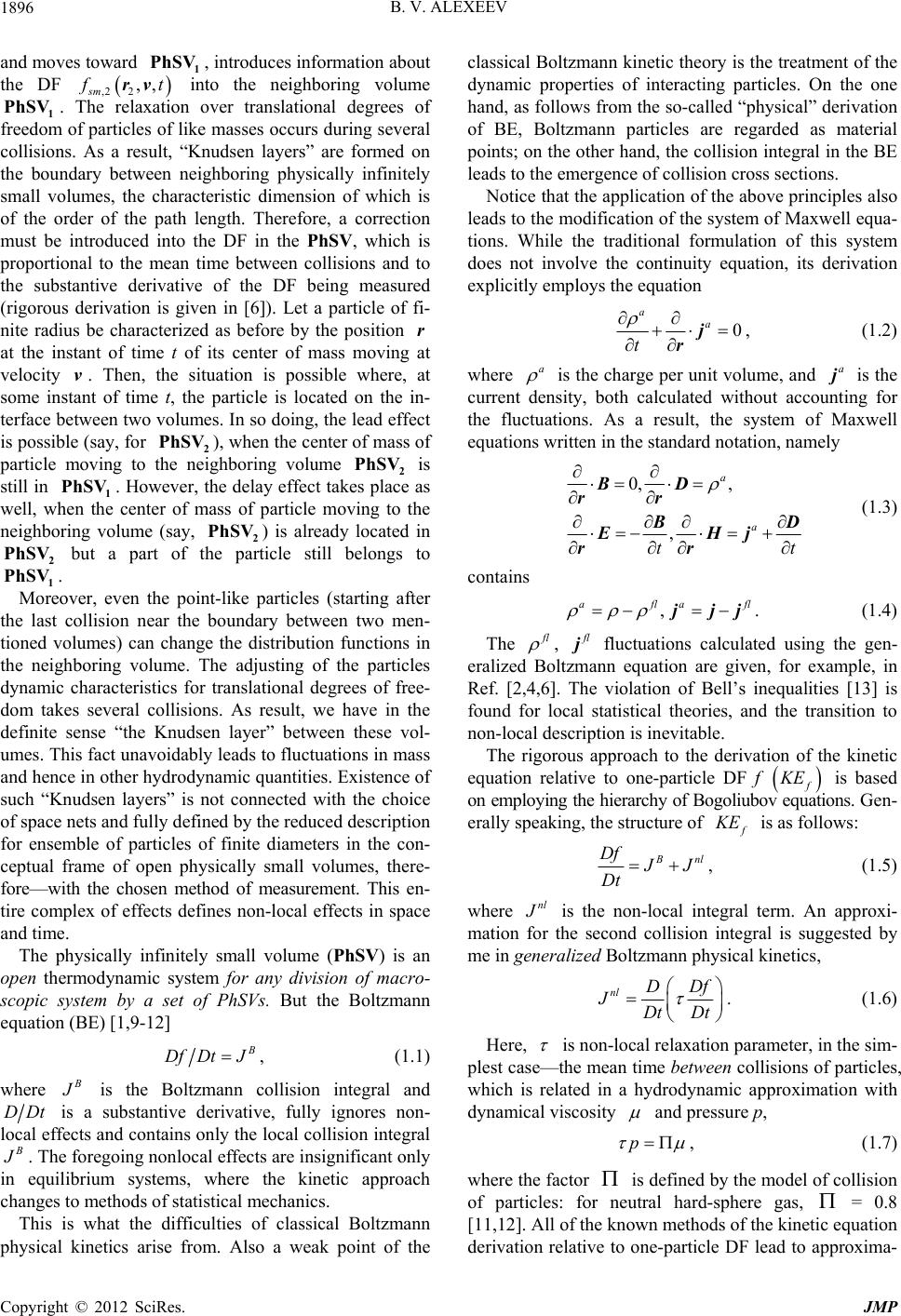 B. V. ALEXEEV 1896 and moves toward 1, introduces information about the DF ,2 2sm PhSV ,, trv r PhSV PhSV PhSV into the neighboring volume 1. The relaxation over translational degrees of freedom of particles of like masses occurs during several collisions. As a result, “Knudsen layers” are formed on the boundary between neighboring physically infinitely small volumes, the characteristic dimension of which is of the order of the path length. Therefore, a correction must be introduced into the DF in the PhSV , which is proportional to the mean time between collisions and to the substantive derivative of the DF being measured (rigorous derivation is given in [6]). Let a particle of fi- nite radius be characterized as before by the position at the instant of time t of its center of mass moving at velocity . Then, the situation is possible where, at some instant of time t, the particle is located on the in- terface between two volumes. In so doing, the lead effect is possible (say, for 2), when the center of mass of particle moving to the neighboring volume 2 is still in 1. However, the delay effect takes place as well, when the center of mass of particle moving to the neighboring volume (say, 2) is already located in but a part of the particle still belongs to . PhSV PhSV PhSV v PhSV 2 1 Moreover, even the point-like particles (starting after the last collision near the boundary between two men- tioned volumes) can change the distribution functions in the neighboring volume. The adjusting of the particles dynamic characteristics for translational degrees of free- dom takes several collisions. As result, we have in the definite sense “the Knudsen layer” between these vol- umes. This fact unavoidably leads to fluctuations in mass and hence in other hydrodynamic quantities. Existence of such “Knudsen layers” is not connected with the choice of space nets and fully defined by the reduced description for ensemble of particles of finite diameters in the con- ceptual frame of open physically small volumes, there- fore—with the chosen method of measurement. This en- tire complex of effects defines non-local effects in space and time. The physically infinitely small volume (PhSV) is an open thermodynamic system for any division of macro- scopic system by a set of PhSVs. But the Boltzmann equation (BE) [1,9-12] DfDt J, (1.1) where is the Boltzmann collision integral and DDt is a substantive derivative, fully ignores non- local effects and contains only the local collision integral . The foregoing nonlocal effects are insignificant only in equilibrium systems, where the kinetic approach changes to methods of statistical mechanics. This is what the difficulties of classical Boltzmann physical kinetics arise from. Also a weak point of the classical Boltzmann kinetic theory is the treatment of the dynamic properties of interacting particles. On the one hand, as follows from the so-called “physical” derivation of BE, Boltzmann particles are regarded as material points; on the other hand, the collision integral in the BE leads to the emergence of collision cross sections. Notice that the application of the above principles also leads to the modification of the system of Maxwell equa- tions. While the traditional formulation of this system does not involve the continuity equation, its derivation explicitly employs the equation 0 a a t j r a , (1.2) where is the charge per unit volume, and is the current density, both calculated without accounting for the fluctuations. As a result, the system of Maxwell equations written in the standard notation, namely a j 0, , , a a tt BD rr D EHj rr , aflaf (1.3) contains l jjj . (1.4) l , The l j fluctuations calculated using the gen- eralized Boltzmann equation are given, for example, in Ref. [2,4,6]. The violation of Bell’s inequalities [13] is found for local statistical theories, and the transition to non-local description is inevitable. The rigorous approach to the derivation of the kinetic equation relative to one-particle DF f E is based on employing the hierarchy of Bogoliubov equations. Gen- erally speaking, the structure of E is as follows: nl Df J Dt nl , (1.5) where is the non-local integral term. An approxi- mation for the second collision integral is suggested by me in generalized Boltzmann physical kinetics, nl DDf JDt Dt . (1.6) Here, is non-local relaxation parameter, in the sim- plest case—the mean time between collisions of particles, which is related in a hydrodynamic approximation with dynamical viscosity and pressure p, p , (1.7) where the factor is defined by the model of collision of particles: for neutral hard-sphere gas, = 0.8 [11,12]. All of the known methods of the kinetic equation derivation relative to one-particle DF lead to approxima- Copyright © 2012 SciRes. JMP 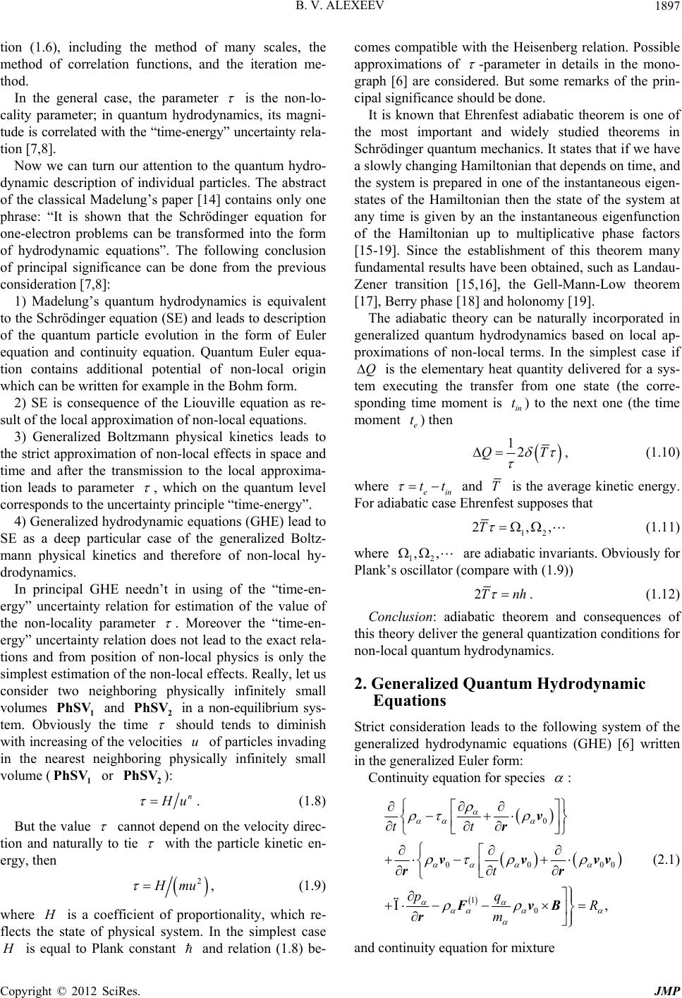 B. V. ALEXEEV 1897 tion (1.6), including the method of many scales, the method of correlation functions, and the iteration me- thod. In the general case, the parameter is the non-lo- cality parameter; in quantum hydrodynamics, its magni- tude is correlated with the “time-energy” uncertainty rela- tion [7,8]. Now we can turn our attention to the quantum hydro- dynamic description of individual particles. The abstract of the classical Madelung’s paper [14] contains only one phrase: “It is shown that the Schrödinger equation for one-electron problems can be transformed into the form of hydrodynamic equations”. The following conclusion of principal significance can be done from the previous consideration [7,8]: 1) Madelung’s quantum hydrodynamics is equivalent to the Schrödinger equation (SE) and leads to description of the quantum particle evolution in the form of Euler equation and continuity equation. Quantum Euler equa- tion contains additional potential of non-local origin which can be written for example in the Bohm form. 2) SE is consequence of the Liouville equation as re- sult of the local approximation of non-local equations. 3) Generalized Boltzmann physical kinetics leads to the strict approximation of non-local effects in space and time and after the transmission to the local approxima- tion leads to parameter , which on the quantum level corresponds to the uncertainty principle “time-energy”. 4) Generalized hydrodynamic equations (GHE) lead to SE as a deep particular case of the generalized Boltz- mann physical kinetics and therefore of non-local hy- drodynamics. In principal GHE needn’t in using of the “time-en- ergy” uncertainty relation for estimation of the value of the non-locality parameter . Moreover the “time-en- ergy” uncertainty relation does not lead to the exact rela- tions and from position of non-local physics is only the simplest estimation of the non-local effects. Really, let us consider two neighboring physically infinitely small volumes 1 and 2 in a non-equilibrium sys- tem. Obviously the time PhSV PhSV should tends to diminish with increasing of the velocities of particles invading in the nearest neighboring physically infinitely small volume ( or ): u 2 PhSV 1 PhSV n u . (1.8) But the value cannot depend on the velocity direc- tion and naturally to tie with the particle kinetic en- ergy, then 2 mu , (1.9) where is a coefficient of proportionality, which re- flects the state of physical system. In the simplest case is equal to Plank constant and relation (1.8) be- comes compatible with the Heisenberg relation. Possible approximations of -parameter in details in the mono- graph [6] are considered. But some remarks of the prin- cipal significance should be done. It is known that Ehrenfest adiabatic theorem is one of the most important and widely studied theorems in Schrödinger quantum mechanics. It states that if we have a slowly changing Hamiltonian that depends on time, and the system is prepared in one of the instantaneous eigen- states of the Hamiltonian then the state of the system at any time is given by an the instantaneous eigenfunction of the Hamiltonian up to multiplicative phase factors [15-19]. Since the establishment of this theorem many fundamental results have been obtained, such as Landau- Zener transition [15,16], the Gell-Mann-Low theorem [17], Berry phase [18] and holonomy [19]. The adiabatic theory can be naturally incorporated in generalized quantum hydrodynamics based on local ap- proximations of non-local terms. In the simplest case if Q is the elementary heat quantity delivered for a sys- tem executing the transfer from one state (the corre- sponding time moment is ) to the next one (the time moment ) then in t e t 12QT tt , (1.10) where ein and T is the average kinetic energy. For adiabatic case Ehrenfest supposes that 12 2,,T ,, (1.11) where 12 are adiabatic invariants. Obviously for Plank’s oscillator (compare with (1.9)) 2Tnh . (1.12) Conclusion: adiabatic theorem and consequences of this theory deliver the general quantization conditions for non-local quantum hydrodynamics. 2. Generalized Quantum Hydrodynamic Equations Strict consideration leads to the following system of the generalized hydrodynamic equations (GHE) [6] written in the generalized Euler form: : Continuity equation for species 0 0000 1 0 I, tt t pq R m v r vvvv rr FvB r (2.1) a nd continuity equation for mixture Copyright © 2012 SciRes. JMP 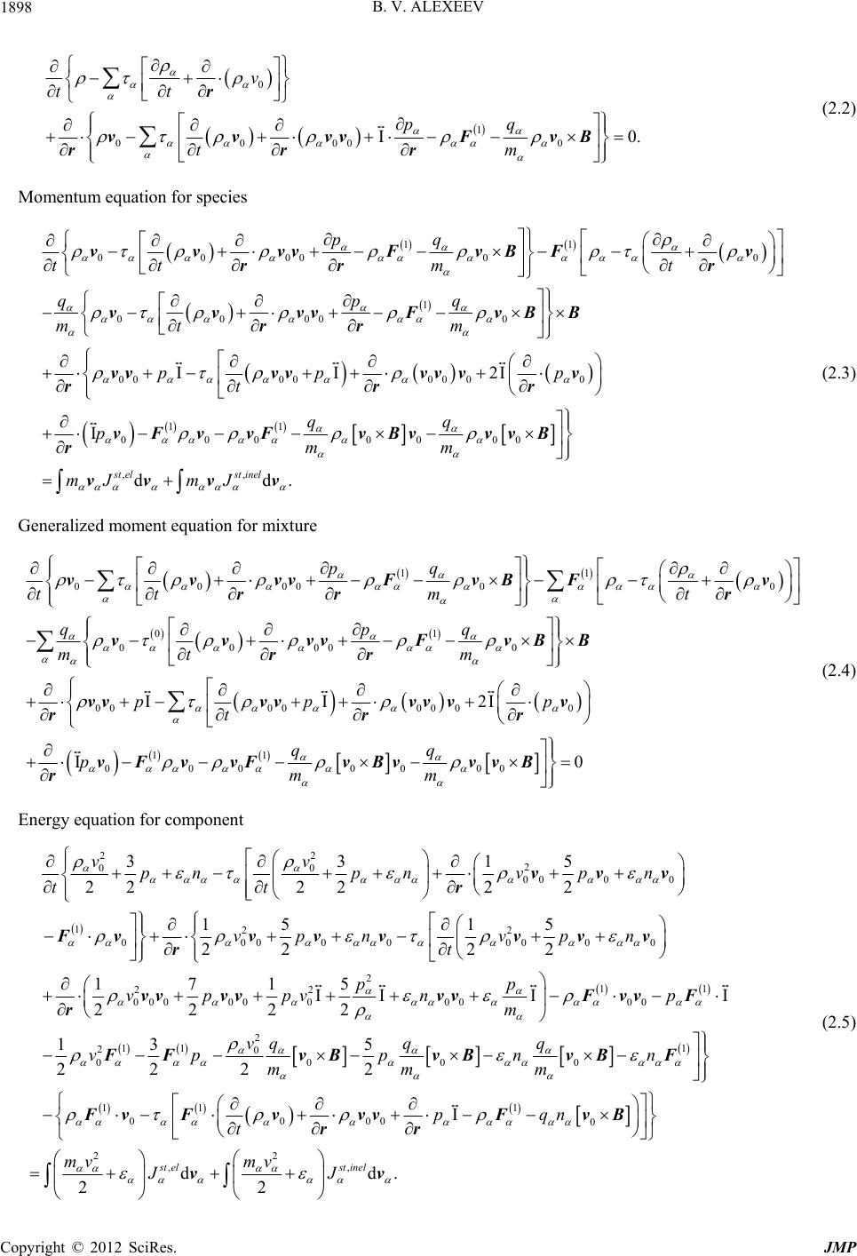 B. V. ALEXEEV Copyright © 2012 SciRes. JMP 1898 0 1 0000 v tt pq tm r vvvvF rrr 0 I0. vB (2.2) Momentum equation for species 11 0000 0 1 0000 0 00 00 I pq tt m qpq mt m pp t 0 t v r vvvvFvBF rr vvvvFvBB rr vv vv r 00 00 11 000 0000 ,, I2I I dd. st elst inel p qq pmm m q m JmJ vv vv rr vF vvFvBvvvB r vv vv (2.3) Generalized moment equation for mixture 11 0000 0 01 0000 0 00 I pq tt m qpq mt m pt 0 t v r vvvvFvBF rr vvvvFvBB rr vv r 0000 00 11 000 0000 I2I I0 q m pp qq pmm vvvv vv rr vF vvFvBvvvB r (2.4) Energy equation for component 22 2 00 00 0 122 0000000 2 000 331 22222 2 15 15 22 22 17 2 vv pnpnv p tt vpn vp t v vv r Fvvvvv v r vv r 0 00 5 n n v v 2 2 00 0000 2 11 20 000 11 1 0000 15 222 13 5 222 2 pp ppvn m vq q q vpp n mmm p t vvvvF v F FvBvBvB Fv FvvvF rr 11 0 1 0 p n v F F 0 22 ,, dd. 22 st elst inel qn mv mv JJ vB vv (2.5) 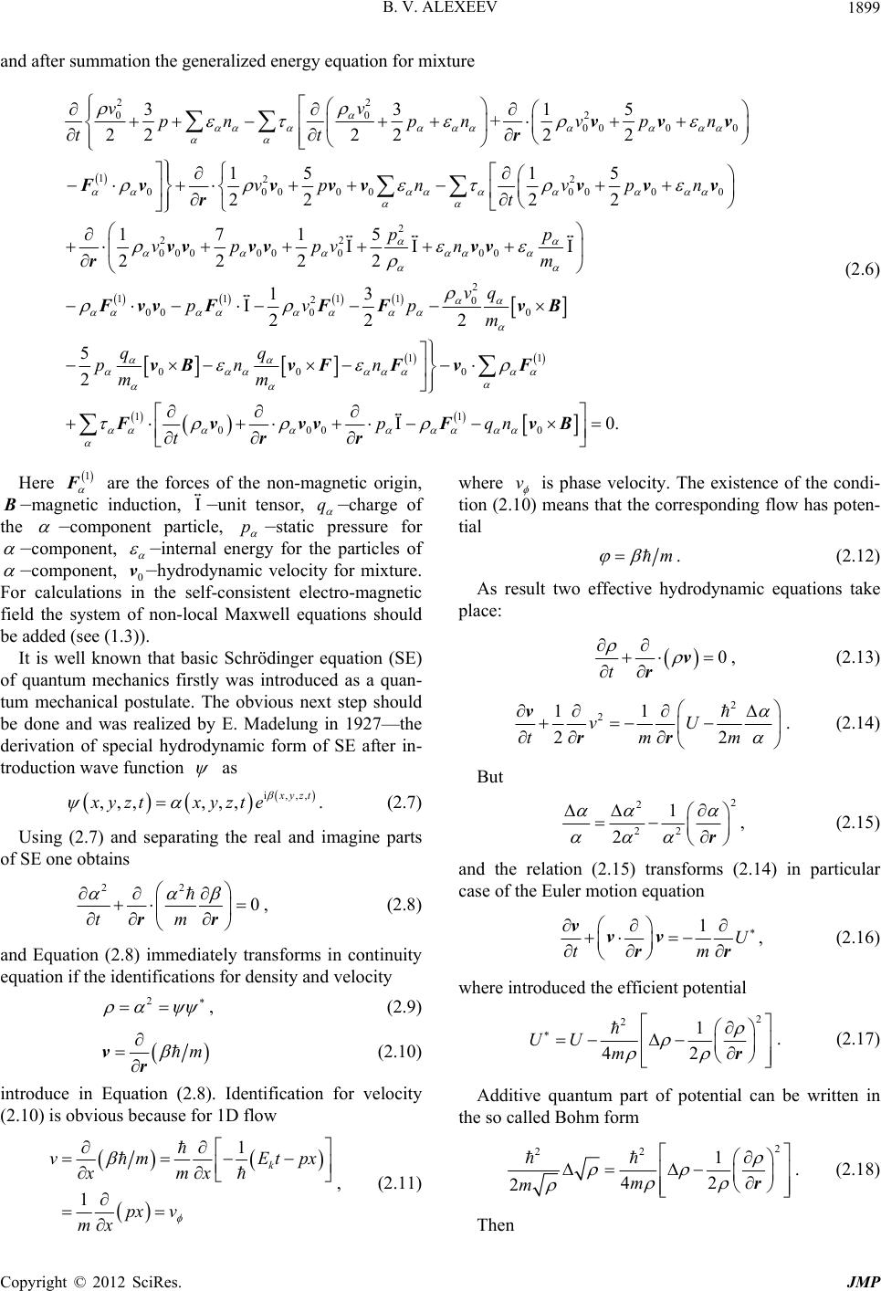 B. V. ALEXEEV 1899 and after summation the generalized energy equation for mixture 22 2 00 00 122 00000 00 2 000 33 + 222 222 151 5 222 2 1 2 vv pnpn v tt vp nv t v r Fv v vvv r vv r 0 0 00 15 p n pn vvv v v 2 2 00 000 2 11 11 20 00 00 11 00 0 1 000 715 222 13 222 5 2 pp ppvn m vq pvp m qq pnn mm p t vv vv Fvv FFFvB vBvFF vF Fvvv rr 1 00.qn FvB (2.6) 1 Here F BIq are the forces of the non-magnetic origin, —magnetic induction, —unit tensor, —charge of the —component particle, p —static pressure for —component, —internal energy for the particles of —component, 0—hydrodynamic velocity for mixture. For calculations in the self-consistent electro-magnetic field the system of non-local Maxwell equations should be added (see (1.3)). v It is well known that basic Schrödinger equation (SE) of quantum mechanics firstly was introduced as a quan- tum mechanical postulate. The obvious next step should be done and was realized by E. Madelung in 1927—the derivation of special hydrodynamic form of SE after in- troduction wave function as ,,, , i,,, ,, yzt zte xyzt xy . (2.7) Using (2.7) and separating the real and imagine parts of SE one obtains 22 0 tm rr 2 , (2.8) and Equation (2.8) immediately transforms in continuity equation if the identifications for density and velocity , (2.9) m r v (2.10) introduce in Equation (2.8). Identification for velocity (2.10) is obvious because for 1D flow 1 vm xm px v mx 1 k Etpx x v , (2.11) where is phase velocity. The existence of the condi- tion (2.10) means that the corresponding flow has poten- tial m. (2.12) As result two effective hydrodynamic equations take place: 0 t v r, (2.13) 2 2 11 22 vU tmm v rr . (2.14) But 2 2 22 1 2 r, (2.15) and the relation (2.15) transforms (2.14) in particular case of the Euler motion equation 1U tm vvv rr , (2.16) where introduced the efficient potential 2 21 42 UU m r . (2.17) Additive quantum part of potential can be written in the so called Bohm form 2 22 1 42 2m m r . (2.18) Then Copyright © 2012 SciRes. JMP 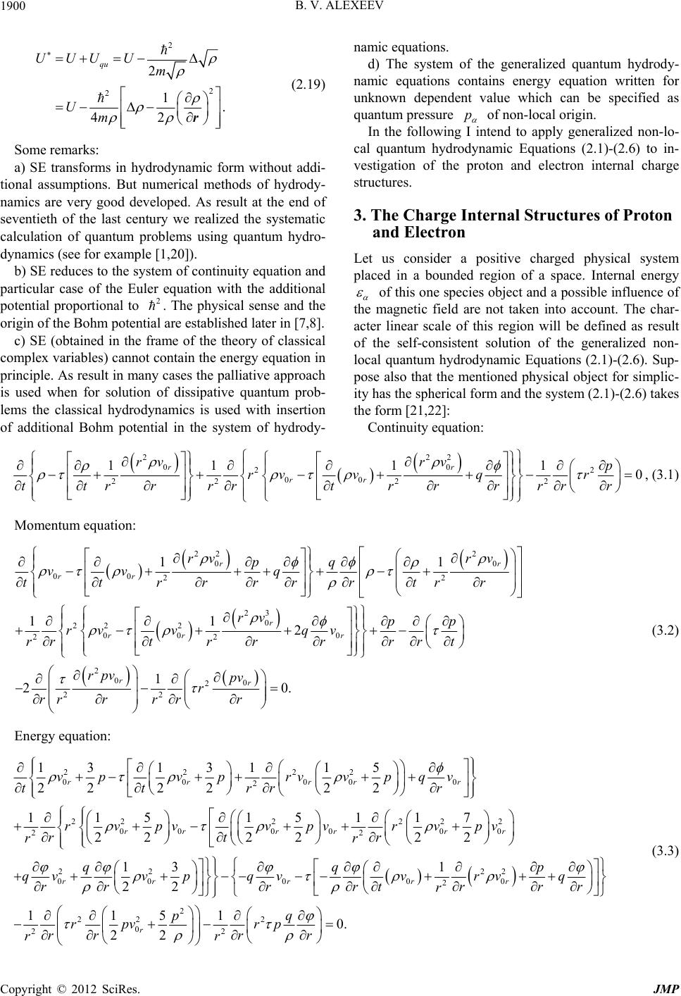 B. V. ALEXEEV 1900 2 2 2 1. 42 m 2 qu UUU U Um r 2 p (2.19) Some remarks: a) SE transforms in hydrodynamic form without addi- tional assumptions. But numerical methods of hydrody- namics are very good developed. As result at the end of seventieth of the last century we realized the systematic calculation of quantum problems using quantum hydro- dynamics (see for example [1,20]). b) SE reduces to the system of continuity equation and particular case of the Euler equation with the additional potential proportional to . The physical sense and the origin of the Bohm potential are established later in [7,8]. c) SE (obtained in the frame of the theory of classical complex variables) cannot contain the energy equation in principle. As result in many cases the palliative approach is used when for solution of dissipative quantum prob- lems the classical hydrodynamics is used with insertion of additional Bohm potential in the system of hydrody- namic equations. d) The system of the generalized quantum hydrody- namic equations contains energy equation written for unknown dependent value which can be specified as quantum pressure of non-local origin. In the following I intend to apply generalized non-lo- cal quantum hydrodynamic Equations (2.1)-(2.6) to in- vestigation of the proton and electron internal charge structures. 3. The Charge Internal Structures of Proton and Electron Let us consider a positive charged physical system placed in a bounded region of a space. Internal energy of this one species object and a possible influence of the magnetic field are not taken into account. The char- acter linear scale of this region will be defined as result of the self-consistent solution of the generalized non- local quantum hydrodynamic Equations (2.1)-(2.6). Sup- pose also that the mentioned physical object for simplic- ity has the spherical form and the system (2.1)-(2.6) takes the form [21,22]: Continuity equation: 222 0 0 2 2 00 222 2 111 1 0 r r rr rvrv p rv vqr ttrrtrrrr rrr r , (3.1) Momentum equation: 22 2 0 0 00 2 2 23 0 222 00 0 22 11 11 2 2 r r rr r rr r rv rv pq vvq tt rrrrtr rr rv pp rv vqv rt rrrrt rr (3.2) 2 00 2 22 10. rr rpv pv r rr rr rr Energy equation: 2222 00 000 2 222222 00 0000 2 2 13 13115 22 2222 115 15117 222222 rr rrr rr rrrr vpvprv vpqv tt rr r r vpvvpvrvpv rtr rr 22 22 00000 2 2 22 2 0 13 1 22 1151 0. rrrrr r qq qvvpqvvrv rrrrt r r pq rpvrp 22 22 p q rr rrr r rr (3.3) Copyright © 2012 SciRes. JMP 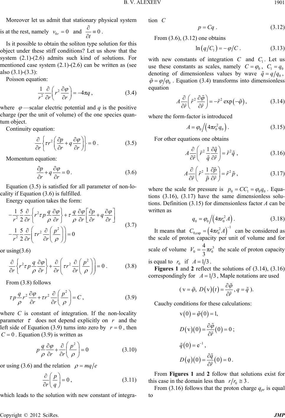 B. V. ALEXEEV 1901 Moreover let us admit that stationary physical system is at the rest, namely and 00 r v0 t . Is it possible to obtain the soliton type solution for this object under these stiff conditions? Let us show that the system (2.1)-(2.6) admits such kind of solutions. For mentioned case system (2.1)-(2.6) can be written as (see also (3.1)-(3.3): Poisson equation: 2 2 1 r4πrq rr , (3.4) where —scalar electric potential and q is the positive charge (per the unit of volume) of the one species quan- tum object. Continuity equation: 2p rr 0rq r . (3.5) Momentum equation: 0 pq rr . (3.6) Equation (3.5) is satisfied for all parameter of non-lo- cality if Equation (3.6) is fulfilled. Energy equation takes the form: 2 2 2 2 2 15 2 15 0 2 qq rp rr r p r rrr p q rrr (3.7) or using(3.6) 2 2 0 p r 2 q rp r rrr . (3.8) From (3.8) follows 2 p C rr 22 q prr , (3.9) where C is constant of integration. If the non-locality parameter does not depend explicitly on and the left side of Equation (3.9) turns into zero by r 0r , then . Equation (3.9) is written as 0C 2 0 p rr q p (3.10) or using (3.6) and the relation mq e 0 p rq С pCq , (3.11) which leads to the solution with new constant of integra- tion . (3.12) From (3.6), (3.12) one obtains 1 ln qC C C C . (3.13) with new constants of integration С and 1. Let us use these constants as scales, namely 0 10 Cq, denoting of dimensionless values by wave 0,qqq 0 . Equation (3.4) transforms into dimensionless equation 22 expAr r rr , (3.14) where the form-factor is introduced 2 000 4π rq . (3.15) For other equations one obtains 22 1q rrq rq r , (3.16) 22 1p rrp rp r pCC q , (3.17) where the scale for pressure is 0100 . Equa- tions (3.16), (3.17) have the same dimensionless solu- tions. Definition (3.15) for dimensionless factor A can be written as 2 000 4πqrA 1 2 4πCrA . (3.18) It means that 0,cap 0 can be considered as the scale of proton capacity per unit of volume and for scale of volume 3 00 4π 3 Vr r the scale of proton capacity is equal to if 013A. Figures 1 and 2 reflect the solutions of (3.14), (3.16) correspondingly for 13A, Maple notations are used (v, vDt r q ,q). Cauchy conditions for these calculations: v00 1, v00 0Dr ; 1 0eq , 000 q Dq r . From Figures 1 and 2 follow that solutions exist for this case in the domain less than 0 From (3.16) follows that the proton charge qpr is equal to 3rr. Copyright © 2012 SciRes. JMP  B. V. ALEXEEV 1902 Figure 1. ,r v= tr r v= for proton, red line r .v= Figure 2. r = for proton. 23 00 00 32 00 0 22 00 00 0 4πd4π 1 4πd d pr pr pr pr or 2 d 1ln r pr rr rqr q rr r rr pr r r qrqrrrq q rqA rr rqr q rrr rqr (3.18) 2ln r pr pr rr q qr r qr (3.19) if ,00 0pr . Relation (3.19) delivers the natural boundary condition for the external area of proton. For example if the restric- tions 0 r rr , 03 0.75 π r r q qr 2 00 pr rq and (there- fore 0 3 4π r r q r ) are introduced then 0 ln 4π 3 pr pr rr pr q q rr ~ (3.20) and in the vicinity of r rr we have 4π exp 3 pr r rr rr qC r 3 . (3.21) Obviously (3.21) can be written using the dimensional (cm ) form-factor q rqpr qr rFq . (3.22) For the chosen scales 0 2 0 1 4π 4πpr Arq . (3.23) As we see the choice of scales is the question of con- venience by the interpretation of the experimental data and the corresponding choice of the Cauchy conditions. Now we can apply the previous theory to the calcula- tion of the internal electron structure. As before we in- tend to consider the electron at the rest placed in the self-consistent intrinsic electric field without an intrinsic magnetic field. In our electron model, we no longer regard the elec- tron as a point-like particle. Similar to the proton’s elec- tric charge, which has continuum distribution inside of the proton, we make the same basic assumptions based on the application of the non-local theory. On this step of investigation no reason to introduce the simplest model of electron spin like a spinning electrically charged ball or much more complicated theory which leads to the magnetic charge continuum distribution inside of the electron using the Dirac monopole speculations [23,24]. Obviously Poisson Equation (3.4) transforms into 2 2 14πrq rr r , (3.24) where —scalar electric potential and is the negative charge (per the unit of volume) of the one spe- cies quantum object. In other words is absolute charge q q Copyright © 2012 SciRes. JMP 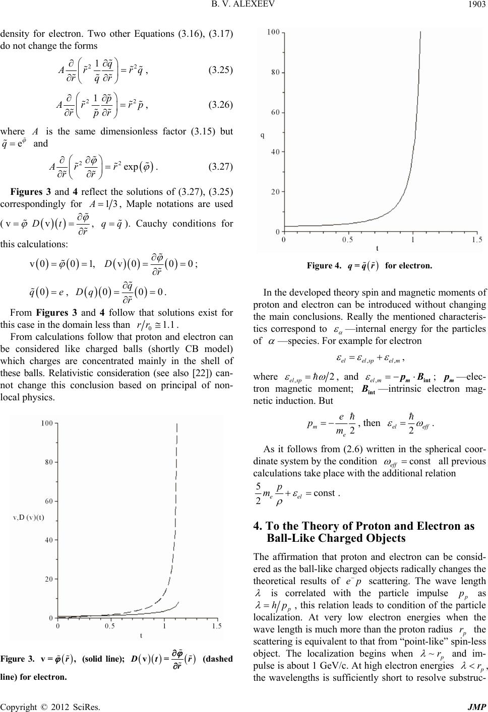 B. V. ALEXEEV 1903 density for electron. Two other Equations (3.16), (3.17) do not change the forms 22 1q rrq rq r , (3.25) 22 1p rrp rp r , (3.26) is the same dimensionless factor (3.15) but where eq and 2 expr 2 Ar rr . (3.27) Figures 3 and 4 reflect the solutions of (3.27), (3.25) correspondingly for 13A, Maple notations are used v (v Dt r qq , ). Cauchy conditions for this calculations: 0 1, v0 0 0 r v0D; 0qe , 000 r q Dq . From Figures 3 and 4 follow that solutions exist for this case in the domain less than 0 From calculations follow that proton and electron can be considered like charged balls (shortly CB model) which charges are concentrated mainly in the shell of these balls. Relativistic consideration (see also [22]) can- not change this conclusion based on principal of non- local physics. 1.1rr . Figure 3. r v= , (solid line); r = for electron. Figure 4. In the developed theory spin and magnetic moments of proton and electron can be introduced without changing the main conclusions. Really the mentioned characteris- tics correspond to —internal energy for the particles of —species. For example for electron ,,elelspel m tr r v= (dashed line) for electron. , where ,el sp2 ,el , and m pBp mint; m—elec- tron magnetic moment; int —intrinsic electron mag- netic induction. But 2 m e e pm , then 2 el eff const . As it follows from (2.6) written in the spherical coor- dinate system by the condition eff all previous calculations take place with the additional relation 5cons t 2eel p m ep . 4. To the Theory of Proton and Electron as Ball-Like Charged Objects The affirmation that proton and electron can be consid- ered as the ball-like charged objects radically changes the theoretical results of scattering. The wave length is correlated with the particle impulse p as hp , this relation leads to condition of the particle localization. At very low electron energies when the wave length is much more than the proton radius r ~ the scattering is equivalent to that from “point-like” spin-less object. The localization begins when r and im- pulse is about 1 GeV/c. At high electron energies r , the wavelengths is sufficiently short to resolve substruc- Copyright © 2012 SciRes. JMP 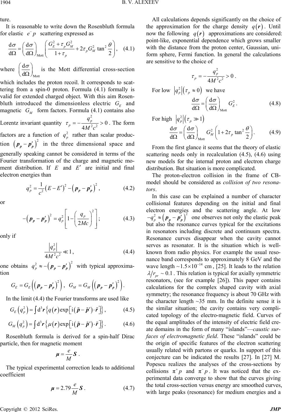 B. V. ALEXEEV 1904 ture. It is reasonable to write down the Rosenbluth formula for elastic scattering expressed as ep 22 Mott dd dd 1 EpM p GG 22 2t an 2 pM G , (4.1) where Mott d d is the Mott differential cross-section which includes the proton recoil. It corresponds to scat- tering from a spin-0 proton. Formula (4.1) formally is valid for extended charged object. With this aim Rosen- bluth introduced the dimensionless electric G and magnetic G form factors. Formula (4.1) contains also Lorentz invariant quantity 2 22 0 4 p q Mc p . The form factors are a function of 2 q rather than scalar produc- tion 2 pp pp E E in the three dimensional space and generally speaking cannot be considered in terms of the Fourier transformation of the charge and magnetic mo- ment distribution. If and are initial and final electron energies than 2 2 2 1 p qE c 2 E pp pp, (4.2) or 2 12 p q Mc 22 p q pp pp ; (4.3) only if 2 22 1 4 p q Mc 2 pp pp 2 , (4.4) one obtains with typical approxima- tion 2 p q 2 pp pp MM GG EE GG , pp pp xpi . In the limit (4.4) the Fourier transforms are used like 23 de Ep Gq q ppr xpi rr , (4.5) 23 de Mp Gq ppr rr . (4.6) Rosenbluth formula is derived for a spin-half Dirac particle, then for magnetic moment e μ . The typical experimental correction leads to additional coefficient . (4.7) All calculations depends significantly on the choice the approximation for the charge of density qr. Until now the following qr approximations are considered: point-like, exponential dependence which gros smaller with the distance from he proton center, Gaussian, uni- form sphere, Fermi function. In general the calculations are sensitive to the choice of w t 2 22 0 4 p p q M c . 20 pp q we have For low 2 dd d Mott dG . (4.8) For high 21 pp q 2.79 e μ 22 Mott dd 12 tan d 2 Mp dG . (4.9) From the first glance it seems that the theo scattering needs only in recalculation (4.5), (4 ne ry of elastic .6) using w models for the internal proton and electron charge distribution. But situation is more complicated. The proton-electron collision in the frame of CB- model should be considered as collision of two resona- tors. In this case can be explained a number of character collisional features depending on the initial and final electron energies and the scattering angle. At low 2 2 p q pp pp c one observes not only the elastic peak but also the resonance curves typical for the excitations in resonators in luding discrete and continuum spectra. Resonance curves disappear when the cavity cannot serves as resonator. It is the situation which is well- known from radio physics. For example the usual reso- nance band corresponds to approximately 8 GeV and the wave length ~14 1.5 10cm , [25]. It leads to the relation ~0.1 pr r . This relation is typical for axially symmetric resonators, (see for example [26]). This paper contains calculations for the complex shaped cavity with axial symmetry; the resonance frequency is about 70 GHz with the character length ~35 mm. In the definite sense it is the similar situation; the cavity contains very compli- cated topology of the electro-magnetic field. Curves of the equal amplitudes of the intensity of electric field cre- ate domains in the form of many “islands”—caustic sur- faces of electromagnetic field. These “islands” could be the origin of specific features of the electron scattering usually related with partons or quarks. In support of this conjecture can be indicated the results [27]. In [27] M. Popescu realizes the analyses of the cross-sections by collisions πp and πp . It was noticed that the ex- perimental data converge to show that the curves giving the total cross-section versus energy are smoothed curves, with large s (resoce) for medium energies and a peaknan Copyright © 2012 SciRes. JMP  B. V. ALEXEEV 1905 slow variation with some waving on the high energy side. Popescu points out that the curves exhibit striking re- semblance to scattering curves obtained by electron, neu- tron or X-ray scattering in liquid and amorphous materi- als. Starting from this observation Popescu developed a method to extract structural information on the proton internal structure, in the hypothesis that ions are scattered by unknown internal centers when they knock the proton. The result of this analysis was very interesting because the total number of scattering centers was estimated as 20 - 30 with the severe variance with the number of quarks now supposed to be integrated in the proton. It should be added that mentioned number of scattering centers is typical for the quantity of “islands” in resonators for the mentioned conditions. In this connection another interesting problem is aris- ing. Can be experimentally confirmed the resonator model for the electron? In this case it is reasonable to remind one old Blokhintsev paper published in Phys- ics-Uspekhi as the letter to Editor [28]. He considered the process of the interaction neutrino and electron e with transformation of electron in -meson: e . In this case the energy density W can be estimated as e Wg , where (4.10) is Fermi constant, ,, e arewave functions for el ectron, -m ng I.S. Sha eson a spondingly ollowipir nd neutrino corre- o, Blokhintsev esti-. F mated as 2 0 gc , (4.11) with 16 10 0~ cm. His conclusion consists in affirm strong interaction place when the ve length ss tha ) c be considered as estim for revealing of the reson hintzev supposes that fulfi ni of the inner charge distribution of the pro- the frame of the non-local quan s to following main results: shell of th ty of el [1] B. V. Alekseev, “Matematicheskaya Kinetika Reagiru- yushchikh Gaz of Reacting Gases, Nauka, Mosco a- tion that the takes of electron and neutrino of the neutrino wa wave pacn 0 . 0 . (4.12) The inequality (4.12an ket le ation ance electron properties. Blo- lling of (4.12) leads to the sig- ficant changes in the Compton effect and to other changes in electro-magnetic interaction of electrons. It is possible also to wait for the influence of the resonance electron effects on investigation of hypothetical neutrino oscillations. 5. Conclusions Investigation ton and electron in hydrodynamics lead tum 1) From calculations follow that proton and electron can be considered like charged balls (shortly CB model) which charges are concentrated mainly in the ese balls. In the first approximation this result does not depend on the choice of the non-locality parameter. The proton-electron collision in the frame of CB- model should be considered as collision of two resona- tors. Curves of the equal amplitudes of the intensi ectric field create domains in proton in the form of many “islands”—caustic surfaces of electromagnetic field which can serve as additional scattering centers. It can open new way for explanation a number of character collisional features depending on the initial and final electron energies without consideration partons or quarks as scattering centers. REFERENCES ov,” Mathematical Theory w, 1982. [2] B. V. Alexeev, “The Generalized Boltzmann Equation, Generalized Hydrodynamic Equations and Their Applica- tions,” Philosophical Transactions of the Royal Society, Vol. 349, 1994, pp. 417-443. doi:10.1098/rsta.1994.0140 [3] B. V. Alexeev, “The Generalized Boltzmann Equation,” Physica A, Vol. 216, No. 4, 1995, pp. 459-468. doi:10.1016/0378-4371(95)00044-8 [4] B. V. Alekseev, “Physical Basements of the Generalized Boltzmann Kinetic Theory of Gases,” Physics Vol. 43, No. 6, 2000, pp. 601-629. -Uspekhi, doi:10.1070/PU2000v043n06ABEH000694 [5] B. V. Alekseev, “Physical Fundamentals of the General- ized Boltzmann Kinetic Theory of ics-Uspekhi, Vol. 46, No. 2, 2003, pp. 139-16 Ionized Gases,” Phys- 7. doi:10.1070/PU2003v046n02ABEH001221 [6] B. V. Alexeev, “Generalized Boltzmann Physical Kinet- ics,” Elsevier, Amsterdam, 2004. [7] B. V. Alexeev, “Generalized Quantum Hydrodynamics and No. 3, 2008, pp. 143- Principles of Non-Local Physics,” Journal of Nanoelec- tronics and Optoelectronics, Vol. 3, 158. doi:10.1166/jno.2008.207 [8] B. V. Alexeev, “Application of Generalized Quantum Hy- drodynamics in the Theory of Quantum Soliton Evolu- tion,” Journal of Nanoelectronics and Optoelectronics, Vol. 3, No. 3, 2008, pp. 316-328. doi:10.1166/jno.2008.311 [9] L. Boltzmann, “Weitere Studien über das Wärmegleich- gewicht unter Gasmolekulen,” Sitzun lichen Akademie der Wissen gsberichte der Kaiser- schaften, Vol. 66, No. 2, 1872, man and T. G. Cowling, “The Mathematical The- p. 275. [10] L. Boltzmann, “Vorlesungen über Gastheorie,” Verlag von Johann Barth, Leipzig, 1912. [11] S. Chap ory of Non-uniform Gases,” Cambridge University Press, Cambridge, 1952. [12] I. O. Hirschfelder, Ch. F. Curtiss and R. B. Bird, “Mo- lecular Theory of Gases and Liquids,” John Wiley and sons, Inc., New York, 1954. Copyright © 2012 SciRes. JMP  B. V. ALEXEEV Copyright © 2012 SciRes. JMP 1906 e Einstein Podolsky Rosen Paradox,” 0, No. 3-4, 1927, pp. 322- [13] J. S. Bell, “On th Physics, Vol. 1, No. 3, 1964, pp. 195-200. [14] E. Madelung, “Quantum Theory in Hydrodynamical Form,” Zeitschrift fur Physik, Vol. 4 325. doi:10.1007/BF01400372 [15] L. D. Landau, “Zur Theorie der Energieübertragung. II,” ty of London A, Vol. 137 tum Physics of the Soviet Union, Vol. 2, 1932, pp. 46-51. [16] C. Zener, “Non-Adiabatic Crossing of Energy Levels,” Proceedings of the Royal Socie , No. 6, 1932, pp. 696-702. [17] M. Gell-Mann and F. Low, “Bound States in Quan Field Theory,” Physical Review, Vol. 84, No. 2, 1951, p. 350. doi:10.1103/PhysRev.84.350 [18] M. V. Berry, “Quantal Phase Factors Accompanying Adia- batic Changes,” Proceedings of the Royal Society of Lon- don A, Vol. 392, No. 1802, 1984, pp. 45-47. doi:10.1098/rspa.1984.0023 [19] B. Simon, “Holonomy, the Quantum Adiabatic Theorem and Berry’s Phase,” Physical Review Letters, Vol. 51, No. 24, 1983, pp. 2167-2170. doi:10.1103/PhysRevLett.51.2167 [20] B. V. Alexeev, A. I. Abakumov and V. S. Vinogradov, “Mathematical Modeling of Elastic Interactions of Fast Electrons with Atoms and Molecules,” Communications on the Applied Mathematics, Computer Centre of the ic Press, 2011. USSR Academy of Sciences, Moscow, 1986. [21] B. V. Alexeev, “Non-Local Physics. Non-Relativistic Theory,” Lambert Academic Press, 2011. [22] B. V. Alexeev and I. V. Ovchinnikova, “Non-Local Phys- ics. Relativistic Theory,” Lambert Academ [23] P. A. M. Dirac, “Quantized Singularities in the Electro- magnetic Field,” Proceedings of the Royal Society of London A, Vol. 133, No. 821, 1931, pp. 60-72. doi:10.1098/rspa.1931.0130 [24] P. A. M. Dirac, “The Theory of Magnetic Mo Physical Reviews, Vol. 74, N nopoles,” o. 7, 1948, pp. 817-830. doi:10.1103/PhysRev.74.817 [25] M. Breidebach, J. I. Friedman, H. W. Kendall, E. Bloom, D. H. Coward, H. DeS D. taebler, J. Drees, L. W. Mo and R. E. Taylor, “Observed Behavior of Highly Inelastic Electron-Proton Scattering,” Physical Review Letters, Vol. 23, No. 16, 1969, pp. 935-939. doi:10.1103/PhysRevLett.23.935 [26] A. Yu. Popkov and I. K. Kuzm with Fragment of Circular Waveguide: Model ichev, “Open Resonator Computa- ol. 57, No. 4, ysics-Uspekhi, Letter to Editor, LXII, tion and Experiment,” Radio-Physics and Radio-As- tronomy, Vol. 14, No. 4, 2009, pp. 425-432. [27] M. Popescu, “Proton Internal Structure Revealed by Pion Scattering,” Romanian Reports in Physics, V 2005, pp. 795-799. [28] D. I. Blokhintsev, “When the Weak Interaction Becomes the Strong One?” Ph Vol. 3, 1957, pp. 381-383.
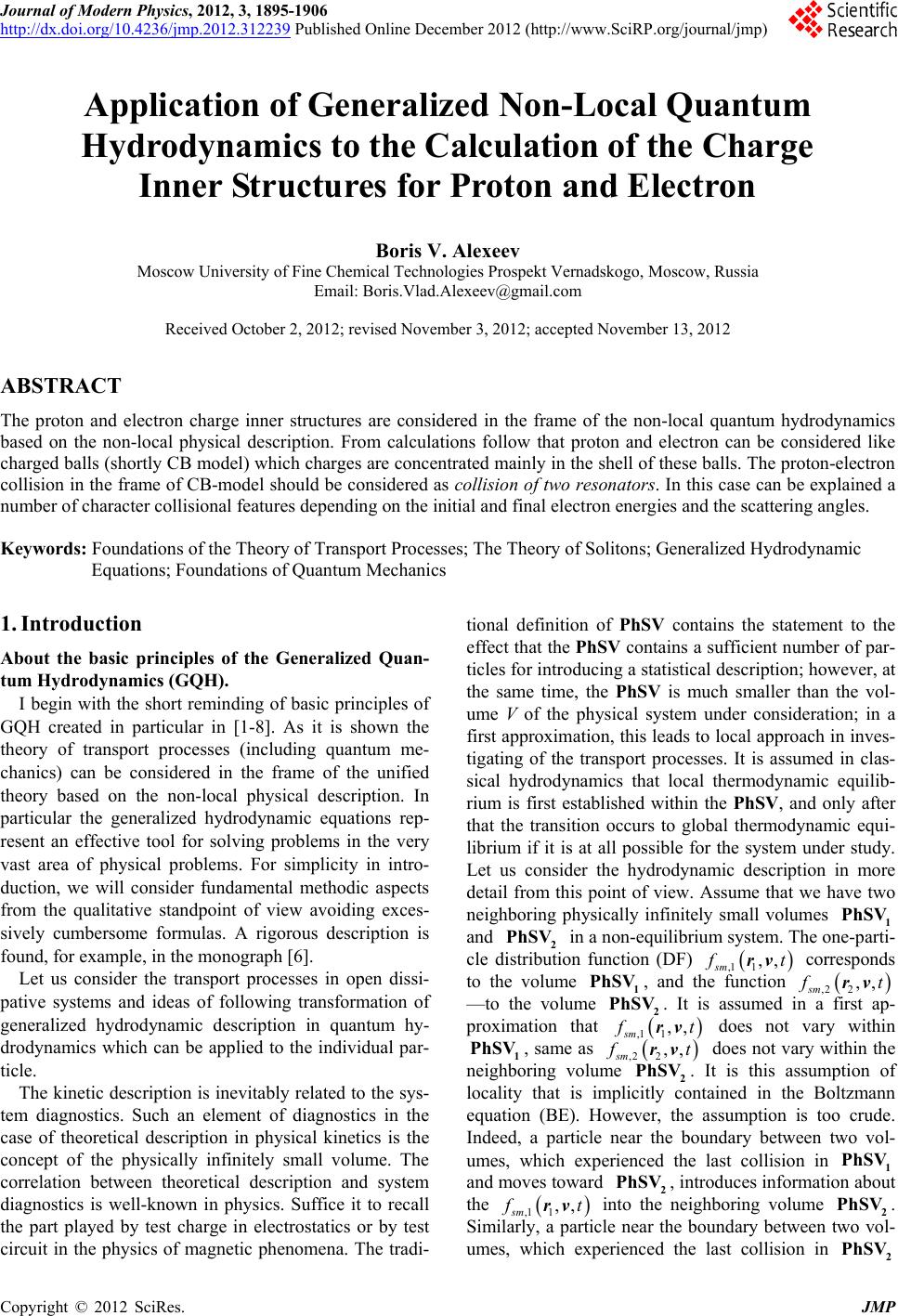
|