American Journal of Computational Mathematics, 2012, 2, 287-294
http://dx.doi.org/10.4236/ajcm.2012.24039 Published Online December 2012 (http://www.SciRP.org/journal/ajcm)
Face Recognition from Incomplete Measurements via
ℓ1-Optimization
Miguel Argaez1*, Reinaldo Sanchez2, Carlos Ramirez2
1Department of Mathematical Sciences, The University of Texas at El Paso, El Paso, USA
2Program in Computational Science, The University of Texas at El Paso, El Paso, USA
Received May 15, 2012; revised August 5, 2012; accepted September 12, 2012
ABSTRACT
In this work, we consider a homotopic principle for solving large-scale and dense underdetermined problems and
its applications in image processing and classification. We solve the face recognition problem where the input image
contains corrupted and/or lost pixels. The approach involves two steps: first, the incomplete or corrupted image is sub-
ject to an inpainting process, and secondly, the restored image is used to carry out the classification or recognition task.
Addressing these two steps involves solving large scale minimization problems. To that end, we propose to solve a
sequence of linear equality constrained multiquadric problems that depends on a regularization parameter that con-
verges to zero. The procedure generates a central path that converges to a point on the solution set of the underde-
termined problem. In order to solve each subproblem, a conjugate gradient algorithm is formulated. When noise is pre-
sent in the model, inexact directions are taken so that an approximate solution is computed faster. This prevents the ill
conditioning produced when the conjugate gradient is required to iterate until a zero residual is attained.
1

1

1

Keywords: Sparse Representation; Minimization; Face Recognition; Sparse Recovery; Interior Point Methods;
Sparse Regularization
1

1. Introduction
Over the last years, new developments in the area of
computational harmonic analysis have shown that a wide
class of signals can be well represented by linear combi-
nations of only few elements of an appropriate basis. The
benefits and applications of this new advance abound and
are of extensive research in the present.
The new sampling theory of compressed sensing has
unified several insights about wavelets and sparse repre-
sentation, benefiting several disciplines in sciences in-
cluding image processing. Practical compressed sensing
problems involve solving an optimization problem of the
form
0
min subject to ,
x
x
Ax b (1)
for decoding a sparse signal that has been sig-
nificantly sub-sampled by a sampling matrix
n
x
mn
A



with Here
.mn0
x
counts the number of non-zero
entries of the vector .
x
Solving (1) is equivalent to finding the sparsest vector
x such that .
A
xb Nevertheless, finding such a vec-
tor x is by nature a combinatorial and generally NP-hard
problem [1]. Efficient numerical algorithms to recover
signals under this framework have been developed [2-4],
and extensions of this theory have been explored for
solving general problems in different areas including
statistics, signal processing, geophysics, and others. Sig-
nificant progress toward understanding this problem has
been made in recent years [5-7], and its study has be-
come state-of-the-art interdisciplinary research.
One of the most important characteristics of problem
(1) is that under some mild conditions, the input vector
x

can be recovered by solving an -norm underde-
termined problem
1

1
min subject to .
x
x
Ax b (2)
This decoding model in compressed sensing is known
as the basis-pursuit problem, first investigated by Chen,
Donoho and Saunders [8] and theoretically studied by
Donoho and Huo [9]. Candès and Tao [5] proved for-
mally this equivalence provided that
x
 is sufficiently
sparse, and that A possesses certain properties.
The compressed sensing theory is extended to solve a
more general problem that considers noise on the meas-
urements, and almost sparsity for the input vector to be
recovered. That is,
*Corresponding author.
C
opyright © 2012 SciRes. AJCM

M. ARGAEZ ET AL. 288
1
min subject to ,
xxAxb

 (3)
where the energy of the noise vector is upper bounded by
.

Problem (3) can also be reformulated as an uncon-
strained regularized linear least-squares problem. One
strategy consists of replacing the Tikhonov regularization
with one that uses the 1-norm [2,4]. Another equiva-
lent formulation is aimed at minimizing the 1 -norm
function regularized by a linear leasts-quares problem [3],
known as unconstrained basis pursuit denoising. All
these approaches have proved to be successful for solv-
ing compressed sensing problems.

We reformulate problem (3) by
1
min subject to ,
x
x
Ax b   (4)
where is bounded by
m
 .

In this work we propose a new strategy to obtain an
optimal solution to problem (4), and present an applica-
tion in robust face recognition to demonstrate the effect-
tiveness of our algorithm. The idea consists of relaxing
the nondifferentiable objective function by a sequence of
multiquadric, continuously differentiable, strictly convex
functions that depend on a positive regularization pa-
rameter .

More precisely, we solve
2
1
min subject to .
n
xi
x
Ax b 


 (5)
The main accomplishment of this idea is that it leads
to the generation of a path that converges to an optimal
solution of problem (4). This leads us to a path-following
algorithm similar to the ones used in primal-dual inte-
rior-point methods. The path-following strategy that we
are proposing uses inexact fixed-point directions to ob-
tain approximate solutions to problems of the form (5).
Such inexact directions are computed via a conjugate
gradient algorithm. In order to prevent the procedure
from becoming costly, a proximity measure to the central
path is introduced for each regularization parameter. The
regularization parameter is defined in a dynamic manner
that converges to zero as in interior-point methods.
2. Problem Formulation
We study the underdetermined problem (4), where
1

m
,
n
x ,b1
1,
n
i
i
x
x

 and
A
is a full-rank
matrix with . The Lagrangian function associated
with problem (4) is
mn
 
T
1
,,lxyxAxb y  
where is the Lagrange multiplier for the equal-
ity constraint. The optimality conditions for (4) are given
by
m
y








T
T
*
T
1 if 0,
1 if 0,
,:
and
1,1 if 0,
i
i
i
nm i
i
i
Ay x
Ay x
Xxy
Ax b
Ay x



 


.


 
















 





Notice that the main role in the characterization of the
optimal conditions for problem (4) is not played by the
Lagrange multiplier ,
y

but by .
T
A
y Using this fact,
the complementarity conditions associated with the pri-
mal variables i
x

are determined by



T
T
0 with 1 if 0
0 with 1 i
.
f 0.
ii ii
i
ii ii
i
xzzA yx
xzzA yx
 
 


 



 


Therefore a necessary condition for a feasible point


,nm xy


 to be an optimal solution of (4) is
T
1
0,0and 0.
n
ii
i
xzxxzA y





 
3. A Regularization Path
The nondifferentiability of (4) is overcome by regulariz-
ing the 1-norm with a sum of continuously differenti-
able functions in the following way: for

0

 suffi-
ciently small,

1 1
n
i
i
x
gx

 where
g
is the scalar
function defined by

2,.
ii i
gx xx 


3.1. Optimality Conditions
We propose to obtain an optimal solution to problem (4)
by solving a sequence of subproblems of the form (5) as
0.


Since each subproblem (5) is strictly convex, then the
optimal solution is obtained by solving the associated
KKT conditions. The Lagrangian function associated
with (5) is
 
T
2
1
,,
n
i
i
lxyxAxb y 


 (6)
where m y

is the Lagrange multiplier for the equal-
ity constraint. Therefore, the KKT conditions are given
by the following square system of nonlinear equations:
 
12 T0
,,
0
Dx xAy
Fxy Ax b











 

(7)
where




2
diag for 1,2,, and 0.
i
Dx xin




3.2. A Fixed Point Problem for the KKT
Conditions
We propose to solve (7) using a fixed-point method. To

M. ARGAEZ ET AL. 289
that effect, we rewrite these nonlinear equations as the
augmented system

12 T0,
0
x
Dx A
yb
A




 


 


 

(8)
where ,
n
x,
m
y



2
diag ,
i
Dx x



1, 2,,,in and 0.


The matrix associated with (8) is nonsingular since
A
has full rank and

12
Dx

 is positive definite. In this
manner, the nonlinear Equation (7) is posed as a fixed-
point problem. In order to solve (8) for a fixed 0,


we proceed by taking an initial point 0
x
and iteratively
compute

,
kkk

x
y   for until two con-
secutive iterations are less than some stopping criteria.
0, 1,k
3.3. Inexact Directions for the Augmented
System
For a current point
_
,
x
the following system

12 T0
_,
0
x
Dx A
yb
A




 


 


 

(9)
is reduced to a weighted normal equation. The first block
of equations gives

12 T
_
0,xDx Ay

 and since
,
A
xb

 we obtain the weighted normal equation

12 T
_
.ADxA yb


  (10)
With this reduction, we move from an indefinite sys-
tem of order to a positive definite system of or-
der Moreover, the conjugate gradient algorithm ap-
plied to (10) converges in at most iterations in exact
arithmetic. The solution
nm
. m
m
x
of (9) is computed directly
by


12 T
_

x
Dx Ay

 once is obtained.
y
Taking into account that the values of T
A
y charac-
terize the optimality set *,
X
we formulate a conjugate
gradient algorithm that finds an approximation of T
A
y
rather than y, see Figure 1.
At each iteration, the CG algorithm satisfies the first
block of equations

12 T
_
0,DxxAy

 therefore
controlling the stopping criteria for solving the aug-
mented system (9) is equivalent to controlling the stop-
ping criteria for solving the linear system 0. Ax b


we define the vector

0, nm r Based on this,

 as the
or for the augmented system, where
.rAxb
residual vect

 Note that 0r

implies
.Ax b

 Now, since

is bounded by ,

then
the conjugate hmgradient algorit stops when
.Ax b

 This implies the stopping criterio
zero, overcoming the ill-conditioning of the
Figure 1. Conjugate gradient algorithm.
4. Path
l path associated with problem (4)
Following Method
4.1. Central Path
We define the centra
by
 
12T 0DxxAy
C

,: .
0
nm
x yAx b
 

















 (11)
The set consists of all the points that are sol
of the sublem (5) for
C
bpro
utions
0.


) as t
This set defines a
smooth cur called the central path that converges to an
optimal solution of problem (4he regularization pa-
rameter
ve

tends to zero [10].
4.2. Promity Measures xi
ollows in the direction
sequencef regularization
Our path-following method f
generated by a decreasing
C
o
parameters

Since moving on C obtain an opti-
mal solution for (4) could be computationally expensive,
we restrict thiterates to some neigorhoods of the cen-
tral path given by
to
e hb
1
:.
1
k
jj
nm
jk
j











 






 (12)
4.3. Updating the Perturbation Parameter

Since T0xz

 is a necessary condition for obtain
optimal solution of problem (4), then following th
ing an
e same
primal-idea ofdual methods we define the regularization
parameter by
n does not
need to be
weighted normal equation close to the solution.
T
,
x
z
  (13)
n
where T ,,
x
xz Ay
1

is the centering pa-

M. ARGAEZ ET AL. 290


0,1 , rameter in andis the
able
n size of the primal vari-
.
x
Tguarantee the decreo ase of the parameter ,

we update it by

p
rev
 where mi  n ,  


0, 1  
and
p
rev

des the pvious value for the regularize-
tion parameter.
Now, we present a globalorithm for so
the convex and nondifferentiable problem (4). The
methodology consists in following the central path C
to
note re
ization alglving
obtain an optimal solution. To prevent the algorithm
from becoming computationally expensive a series of
neighborhoods, ,
k


around the central path are de-
fined to be used as proximity measures of the path for a
decreasing regularization parameters .

To obtain an
approximate solution on the path for a given 0,

 an
inexact fixed-point procedure is applied to (8) until a
point

,.xy



If an optimal solution to (4) is not
found, we decrease ,

specify a new neighborhood


and repeat the fixed-point procedure. An optimal
solutiofound as , n for (4) is

approaches to zero. For
the primal variables
x
 we define their corresponding
complementarity variables z
 such that 0
ii
xz

 and
0
i
z
 for 1, ,in at the optimal solution of prob-
lem (4). This allows us to define the regularization pa-
rameter

in the same manner as in interior-point
methods.
4.4. Path Following Algorithm
In this sec
ry” (
tion we
PFSR prese t our “Path-
) algo ithm. The pseu
2.
n
r
Following
Recove do-cod
Sign
e for
al
m of
the algorithm is presented in Figure
The PFSR algorithm generates two sequences of iter-
ates. The first sequence (inner loop) generates a series of
iterates for obtaining an approximate solution of sub-
problem (5) for a fixed regularization parameter 0.


The second sequence (outer loop) generates a series of
approximate solutions for the subproblem (5) that con-
verges to an optimal solution of problem (4) for a se-
quence of decreasing regularization parameters 0.


5. Sparse Signal Recovery
In this section, we present a set of experimentltal res
AB im
us
ple-that illustrate the performance of th
m.
e MATL
mentation for the proposed algorith
In the implementation of Algorithm 1 the initial points
and the parameters are chosen as follows. In Step 1a, the
initial points for T
Ay
and
x
are the n-dimensional
zero vector. In Step 2, we fix the maximum number of
CG iterations by cg_maxiter = 10.
In the implementation of Algorithm 2 the parameters
are chosen as follows. The initial regularization parame-
ter

is given by

T
1,
n
ii
1i
x
Ab  


Figure 2. PFSR algorithm.
where
x
is the minimum energy reconstruction. Our
numperimentation suggests erical ex0.008


0 as the
(5) to
m
as a
In Step 3, we axi-
umber o solve.
good choice.
num
set maxiter = 1
f subproblems of the formm
The new regularization parameter

is updated in Step
10 by


min ,gap

  with 0.9.


5.1. Sparse Signal Recovery Example
This experimentation has the objeive of investigating
the capg sparse
ct
ability of recoverin signals by our PFSR
algorithm. The goal in this test is to reconstruct a
re m < n. length-n sparse signal from m observations, whe
We start with a classical example also considered in
[2,4,11]. The problem consists of recovering a signal
4096
x with 160 spikes with amplitude ±1, from m =
1024 noisy measurements. We use a partial DCT matrix
A whose m rows are chosen randomly from the nn

discrete cosine transform, without having access to it in
explicit form, but using A as a linear operator on .
n

The same for the matrix T.
A
Partial DCT matrices are
fast transforms for which matrix-vector multiplications
cost just


logOn n flops, and storage is not required.
This case is common for compressed sensing [3,4].
this problem, we have ,
m
Ax   where the
noise vector
In
b

is set according to a Gaussian distribu-
tion with mean 0 an standard deviation 0.01. The origin-
nal and reconstructed signal are shown in Figure 3.
Moreover, the algorithm was successfully run one hun-
dred times wit an average CPU time of 0.2895 seconds,
and 0.0491 average relative 2-norm error defined by
d
h
2
2
2-norm error ,
xx
x




being
x

the true solution and x the solution reached by
m. the PFSR algorith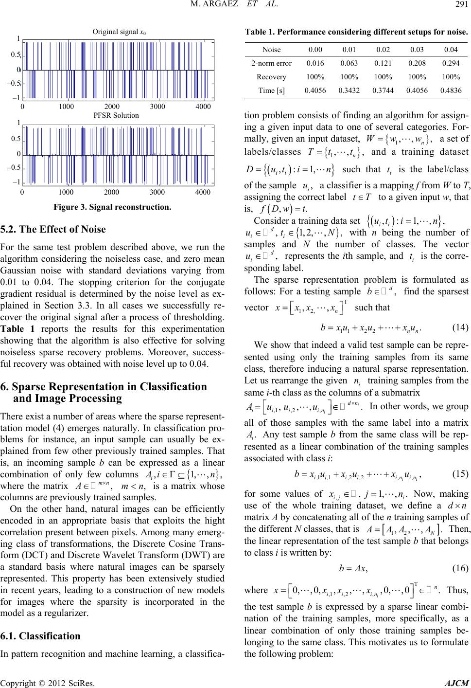

M. ARGAEZ ET AL. 291
Original signal x
0
1
0.5
0
–0.5
–1
1
0.5
0
–0.5
–1
0 1000 2000 3000 4000
PFSR Solution
0 1000 2000 3000 4000
Figure 3. Signal reconstruction.
5.2. The Effect of Noise
For the same test problem described above, we run the
algorithm considering the noiseless case, and zero mean
Gaussian noarying from
0.01 to 0.04. The stopping criterion for the conjugate
ed by the noise level as ex-
ro-
blems for instance, an input sample can usually be ex-
at
is, be expressed as a linear
ise with standard deviations v
gradient residual is determin
plained in Section 3.3. In all cases we successfully re-
cover the original signal after a process of thresholding.
Table 1 reports the results for this experimentation
showing that the algorithm is also effective for solving
noiseless sparse recovery problems. Moreover, success-
ful recovery was obtained with noise level up to 0.04.
6. Sparse Representation in Classification
and Image Processing
There exist a number of areas where the sparse represent-
tation model (4) emerges naturally. In classification p
plained from few other previously trained samples. Th
an incoming sample b can
combination of only few columns


,1,,,
i
A
in 
where the matrix ,
mn
A  ,mn is a matrix whose
columns are previously trained samples.
On the other hand, natural images can be efficiently
encoded in an appropriate basis that exploits the hight
correlation present between pixels. Among many emerg-
ing class of transformations, the Di crete Cosine Trans-
form (DCT) and Discrete Wavelet Transform (DWT) are
a
s
0.01 0.02 0.03 0.04
standard basis where natural images can be sparsely
represented. This property has been extensively studied
in recent years, leading to a construction of new models
for images where the sparsity is incorporated in the
model as a regularizer.
6.1. Classification
In pattern recognition and machine learning, a classifica-
Table 1. Performance considering different setups for noise.
Noise 0.00
2-norm error0.016 0.063 0.121 0.208 0.294
Recovery %100 %100 %100 %100 %100
Time [s] 0.40560.3432 0.3744 0.40560.4836
tion m consists ofng rior -
innpa tofal rie
ma andaf
labels/classes
proble findian algothm fassign
g a given iut dato one severcategos. For-

1
w

,
n
w, ,W lly, given input taset, a set o


, ,
n
t
1,tT trg and a ainindataset




,: 1,ti n
ii i
of the sample ,
i
u a classifier is a mapping f from W to T,
assigning the correct label tT tout w, that
is,
Du such that is the label/class
a given inp
t


,.
f
Dw t

Consider a tra

inin


,: 1,,,
ii
ut in g data set


,1,2,,
d
ii
ut N
N
, with n being the number of
samples and the number of classes. The vector
,
d
i
u

represents the ith sample, and i t is the corre-
sponding label.
The sparse representation p
ple ,
d
b find the sparsest
vector T
12,
,,
n
roblem is formulated as
follows: For a testing sam
x
xx x

 


 such that
112 2. nn
bxu xuxu

 (14)
sampl
erefore inducing arse representation.
rrange the given samples from the
same i-th class as the colums of a submatrix
We show that indeed a valid test sample can be repre-
sented using only the traininges from its same
class, th natural spa
Let us reatraining
i
n
n
,1 ,2,
,,, .
i
i
dn
iii in
uu u



 In other words, we group
all of those samples with the same label into a matrix
.
i
A
A
Any test sample b from the same class will be rep-
resented as a linear combination of the training samples
associated with class i:
,1 ,1,2,2iii i
bxuxu,, ,
inin
xu
ii

 (15)
for some values of ,,1,,.
ij i
x
jn

 Now, making
use of the whole training dataset, we define a dn

matrix A by concatenating all of the n training samples of
the different N classes, that is


12
,,, .
N
A
AA
entation of the test sample
A
b t
Then,
the linear repres
:
hat belongs
to class i is written by
,bAx

()
where T
,1, 2
0, ,0,,, ,,0
ii
xxx



 Thus,
the test sample b is expressed by a sparse linear combi-
nation of the training
16




samples, more specifically, as a
linear combination of only th
longing to the same class. This motivates us to formulate
the following problem:
,, ,0.
i
n
in
x
ose training samples be-

M. ARGAEZ ET AL. 292
1
minsubject to ,
x
Ax b (17)
follows the same structure as (2).
.
6.1.1. Discrimi n a nt Functions and Classifier
s computed, we
which
One of the advantages of this formulation is that the
lack of robustness with respect to outliers can be over-
come. Furthermore, we do not need to care for model
selection as in support vector machine approaches for
classification problems [13]
Once the sparse representation vector x i
identify the class to which the testing sample b belongs.
The approach consists in associating the nonzero entries
of x with the columns of A corresponding to those train-
ing samples having the same class of the testing sample b.
The solution vector x is decomposed as the sum of
d-dimensional vectors ˆ,
k
x
where ˆk
x
is obtained by
h class k keeping only those entries in x associated wit
and assigning zeros to all the other entries. Then, we de-
fine the N discriminant functions

2
ˆ,1,,.
kk
g
bbAxkN  (18)
Thus, k
g
represents the approximation error when b
is assigned to category k. Finally, we assign b to the class
with the smallest approxition error. That is, ma



ˆarg min,1,,.
k
tgbkN (19)
In this manner, we identify the class of the test sample
b based on how effectively the coefficients as
with the training samples of each class recreate b.
red by its
error rate on the entire population. Cross Valida
statistical method for evaluating performance i
th
eing validated.
sociated
6.1.2. Cross Valid ation
A classifier performance is commonly measu
tion is a
n which
e data is divided in two sets: one used for the training
stage, and the second one used for testing (validation).
Both training and testing sets should cross-over in con-
secutive rounds in such a way that each sample in the
data set has a chance of b
In the case of K-fold cross validation, a K-fold parti-
tion of the dataset is created by splitting the data into K
equally (nearly equal) sized subsets (folds), and then for
each of the K experiments, K − 1 folds are used for
training and the remaining one for testing. A common
choice for K-Fold cross validation is K = 10. The work in
[12], compares several approaches for estimating accu-
racy, and recommends stratified 10-fold cross-validation
as the best model selection method because it provides
less biased estimation of the actual accuracy. In our nu-
merical experimentation we follow this validation ap-
proach to test the performance of the classification algo-
rithm.
6.2. Image Processing
In many practical image processing applications, we are
interested in recover a target image ,
n
u that has
been subject to a degradation processes modeled as
,bHu


 (20)
where m b

is the degraded image,

is additive
noise of certain distribution, and H is a linear operator
that acts on the target image u. For instance, H can be a
odels atmospheric turbulence,
n process due to movement.
whic
the image. Consequently, addition
in orde
convolution operator that m
or defects on the acquisitio
From a point of view of parameter estimation, problem
(20) corresponds to an inverse problemh is very
difficult to solve due to the ill-conditioning nature of H
and the large number of degrees of freedom present in
al information is re-
quired r to obtain a meaningful solution to (20).
This is accomplished with the 1  norm regularization,
and our problem becomes
1
minsubject to ,
x
x
Hx b    (21)
where

is an sparsifying matrix for u, and x is a
sparse vector of coefficients. That is, .ux
When H models a process of missing information, it
receives the name of mask, and is constructed by remov-
ing from the nn

identity matrix, the n − m rows asso-
ciated with the missing data. In this setting, we consider
that n − m pixels has been lost, leading to an incomplete
image .
m
b

7. Robust Face Recognition
rrupd.
man faces from the
ambridge University
In this section, we demonstrate the effectiveness of the
proposedlgorithm by showing a rea al application in ro-
bust face recognition. The challenge consists in auto-
matically identify an input human face image within an
existing database of several individuals [14]. Further-
more, we assume that the input image has been subject to
a data loss process, or that several of its pixels has been
severely cote
We consider the database of hu
AT&T laboratories in Cambridge (C
Computer Laboratory)1 which consists of 400 images of
40 individuals each of which with ten different images.
For some individuals, the images were taken at different
times, lighting and facial expression. The size of each
image is 112 92

pixels with 256 gray levels in a pgm
format.
The proposed approach involves two steps. First, the
test image containing several corrupted or lost pixels is
reconstructed via inpainting. To that end, we solve prob-
lem (21) where b is the corrupted test image,

is the
wavelet Daubechies level 7 matrix, and H is the matrix
1http://www.cl.cam.ac.uk/research/dtg/attarchive/facedatabase.html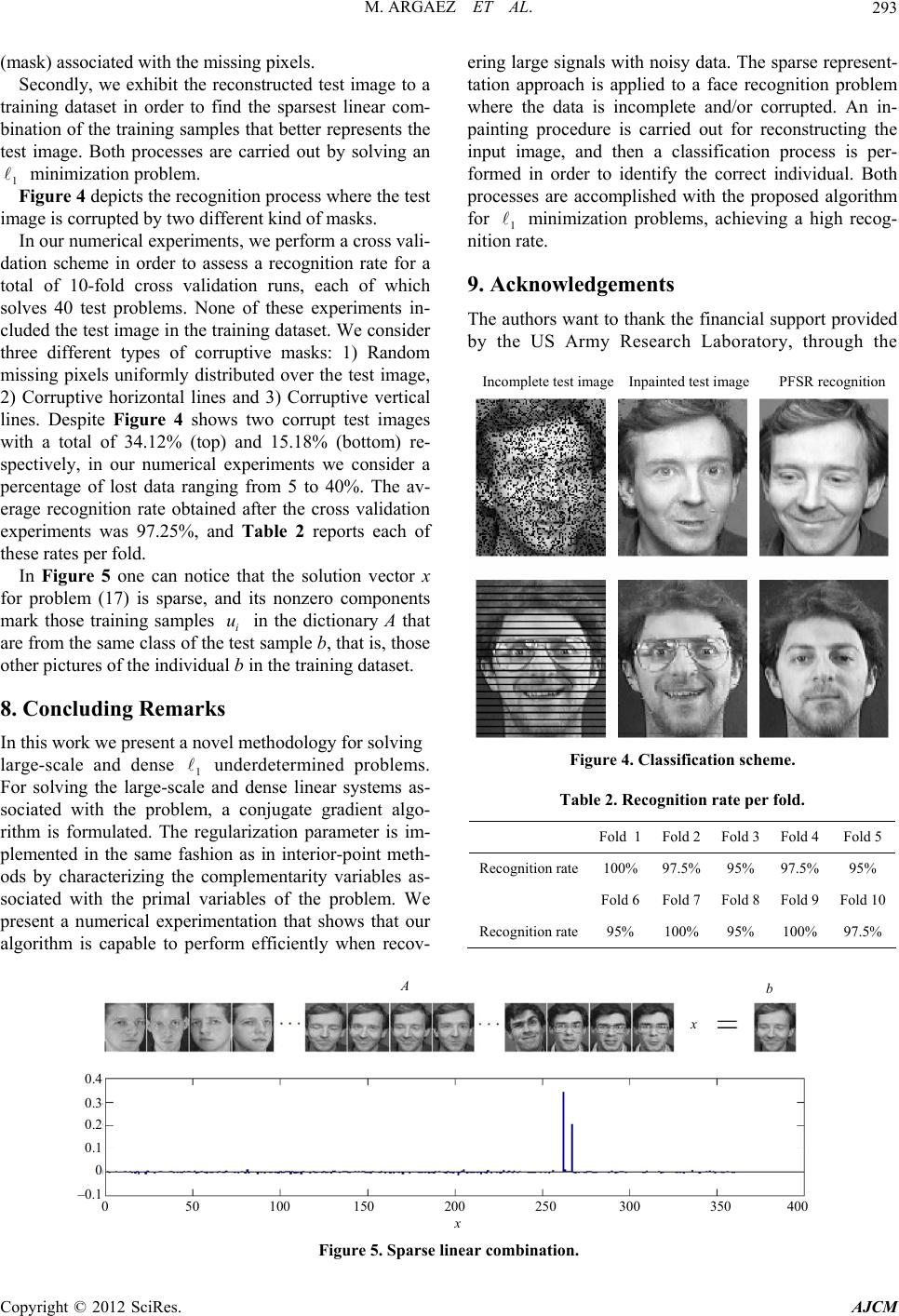

M. ARGAEZ ET AL. 293
f the tra
e. Both processes are carried out by solving an
ro
ach of which
so
2)s and 3) Corruptive vertical
lin
) re-
sp
e
tation that shows that our
efficiently when recov-
ering large signals with noisy data. The sparse represent-
tation approach is applied to a face recognition problem
where the data is incomplete and/or corrupted. An in-
painting procedure is carried out for reconstructing the
input image, and then a classification process is per-
formed in order to identify the correct individual. Both
processes are accomplished with the proposed algorithm
for 1 minimization problems, achieving a high recog-
nition rate.

(mask) associated with the missing pixels.
Secondly, we exhibit the reconstructed test image to a
training dataset in order to find the sparsest linear com-
bination oining samples that better represents the
test imag
1 minimization problem.
Figure 4 depicts the recognition process where the test
image is corrupted by two different kind of masks.
In our numerical experiments, we perform a css vali-
dation scheme in order to assess a recognition rate for a
total of 10-fold cross validation runs, e

lves 40 test problems. None of these experiments in-
cluded the test image in the training dataset. We consider
three different types of corruptive masks: 1) Random
missing pixels uniformly distributed over the test image,
Corruptive horizontal line
9. Acknowledgements
The authors want to thank the financial support provided
by the US Army Research Laboratory, through the
Incomplete test image Inpainted test image PFSR recognition
es. Despite Figure 4 shows two corrupt test images
with a total of 34.12% (top) and 15.18% (bottom
ectively, in our numerical experiments we consider a
percentage of lost data ranging from 5 to 40%. The av-
erage recognition rate obtained after the cross validation
experiments was 97.25%, and Table 2 reports each of
these rates per fold.
In Figure 5 one can notice that the solution vector x
for problem (17) is sparse, and its nonzero components
mark those training samples i u in the dictionary A that
are from the same class of the test sample b, that is, those
other pictures of the individual b in the training dataset.
8. Concluding Remarks
In this work we present a novel methodology for solving
large-scale and dense  underdetermined problems.
Fo
Figure 4. Classification scheme.
1
r solving the large-scale and dense linear systems as-
sociated with the problem, a conjugate gradient algo-
rithm is formulated. The regularization parameter is im-
plemented in the same fashion as in interior-point meth-
ods by characterizing the complementarity variables as-
sociated with the primal variables of the problem. W
Table 2. Recognition rate per fold.
Fold 1Fold 2 Fold 3 Fold 4Fold 5
Recognition rate100%97.5% 95% 97.5%95%
Fold 6Fold 7 Fold 8 Fold 9Fold 10
Recognition rate
present a numerical experimen
algorithm is capable to perform %95 %100 %95 %100 %97.5
x
b
0.4
0.3
0.2
0.1
0
–0.1
A
0 50 100 150 200 250 300 350 400
x
Figure 5. Sparse linear combination.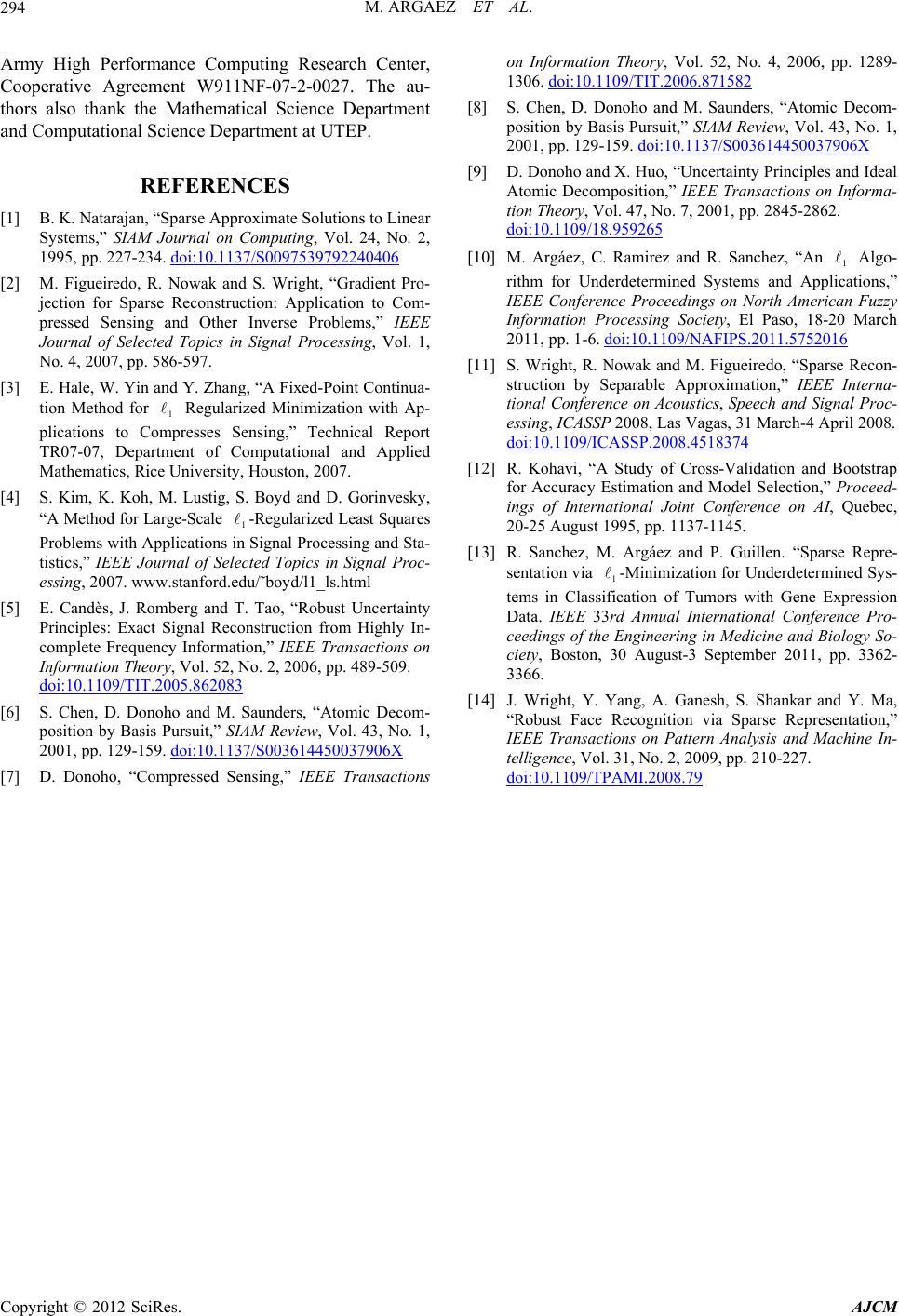

M. ARGAEZ ET AL. 294
Army High Performance Computing Research Center,
Cooperative Agreement W911NF-07-2-0027. The au-
thors also thank the Mathematical Science Department
and Computational Science Department at UTEP.
REFERENCES
[1] B. K. Natarajan, “Sparse Approximate Solutions to Linear
Systems,” SIAM Journal on Computing, Vol. 24, No. 2,
1995, pp. 227-234. doi:10.1137/S0097539792240406
on Information Theory, Vol. 52, No. 4, 2006, pp. 1289-
1306. doi:10.1109/TIT.2006.871582
[8] S. Chen, D. Donoho and M. Saunders, “Atomic Decom-
position by Basis Pursuit,” SIAM Review, Vol. 43, No. 1,
2001, pp. 129-159. doi:10.1137/S003614450037906X
[9] D. Donoho and X. Huo, “Uncertainty Principles and Ideal
Atomic Decomposition,” IEEE Transactions on Informa-
tion Theory, Vol. 47, No. 7, 2001, pp. 2845-2862.
doi:10.1109/18.959265
[10] M. Argáez, C. Ramirez and R. Sanchez, “An Algo-
rithm for Underdetermined Systems and Applications,”
IEEE Conference Proceedings on North American Fuzzy
Information Processing Society, El Paso, 18-20 March
2011, pp. 1-6. doi:10.1109/NAFIPS.2011.5752016
[2] M. Figueiredo, R. Nowak and S. Wright, “Gradient Pro-
jection for Sparse Reconstruction: Application to Com-
pressed Sensing and Other Inverse Problems,” IEEE
Journal of Selected Topics in Signal Processing, Vol. 1,
No. 4, 2007, pp. 586-597.
] E. Hale, W. Yin and Y. Zhang, “A Fixed
[4] S. Kim, K. Koh, M. Lustig, S. Boyd and D. Gorinvesky
“A Method forrized Least Squares
Problems with rocessing and Sta-
[3 -Point Continua-
tion Method for 1  Regularized Minimization with Ap-
plications to Compresses Sensing,” Technical Report
TR07-07, Department of Computational and Applied
Mathematics, Rice University, Houston, 2007.
,
Large-Scale 1 -Regula
Applications in Signal P
tistics,” IEEE Journal of Selected Topics in Signal Proc-
essing, 2007. www.stanford.edu/˜boyd/l1_ls.html
[5] E. Candès, J. Romberg and T. Tao, “Robust Uncertainty
Principles: Exact Signal Reconstruction from Highly In-
complete Frequency Information,” IEEE Transactions on
Information Theory, Vol. 52, No. 2, 2006, pp. 489-509.
doi:10.1109/TIT.2005.862083
[6] S. Chen, D. Donoho and M. Saunders, “Atomic Decom-
position by Basis Pursuit,” SIAM Review, Vol. 43, No. 1,
2001, pp. 129-159. doi:10.1137/S003614450037906X
[7] D. Donoho, “Compressed Sensing,” IEEE Transactions
1

. Nowak and M. Figueiredo, “Sparse Recon-
Separable Approximation,” IEEE Interna-
[11] S. Wright, R
struction by
tional Conference on Acoustics, Speech and Signal Proc-
essing, ICASSP 2008, Las Vagas, 31 March-4 April 2008.
doi:10.1109/ICASSP.2008.4518374
[12] R. Kohavi, “A Study of Cross-Validation and Bootstrap
for Accuracy Estimation and Model Selection,” Proceed-
ings of International Joint Conference on AI, Quebec,
20-25 August 1995, pp. 1137-1145.
[13] R. Sanchez, M. Argáez and P. Guillen. “Sparse Repre-
sentation via 1
-Minimization for Underdetermined Sys-
tems in Classification of Tumors with Gene Expression
Data. IEEE 33rd Annual International Conference Pro-
ceedings of the Engineering in Medicine and Biology So-
ciety, Boston, 30 August-3 September 2011, pp. 3362-
3366.
[14] J. Wright, Y. Yang, A. Ganesh, S. Shankar and Y. Ma,
“Robust Face Recognition via Sparse Representation,”
IEEE Transactions on Pattern Analysis and Machine In-
telligence, Vol. 31, No. 2, 2009, pp. 210-227.
doi:10.1109/TPAMI.2008.79