Journal of Modern Physics, 2012, 3, 1882-1890
http://dx.doi.org/10.4236/jmp.2012.312237 Published Online December 2012 (http://www.SciRP.org/journal/jmp)
Wavefronts and Light Cones for Kerr Spacetimes
Francisco Frutos-Alfaro1, Frank Grave2, Thomas Müller2, Daria Adis3
1Department of Physics, University of Costa Rica, San Pedro, Costa Rica
2Institute for Visualization und Interactive Systems, University of Stuttgart, Stuttgart, Germany
3Theoretical Astrophysics, University of Tübingen, Tübingen, Germany
Received September 26, 2012; revised October 27, 2012; accepted November 5, 2012
ABSTRACT
We investigate the light propagation by means of simulations of wavefronts and light cones for Kerr spacetimes. Simu-
lations of this kind give us a new insight to better understand the light propagation in presence of massive rotating black
holes. A relevant result is that wavefronts are backscattered with winding around the black hole. To generate these
visualizations, an interactive computer program with a graphical user interface, called JWFront, was written in Java.
Keywords: General Relativity; Wavefronts; Lightcones; Simulations
1. Introduction
In general relativity and astrophysics, Kerr spacetimes
are useful to study, for example, stellar compact objects,
like accretion disks in neutron stars. This metric was
found by Kerr in 1963 [1], since then this spacetime ap-
pears in many articles on these topics and it is currently
one of the most used metric, because this represents a
spacetime of a massive rotating object.
Friedrich and Stewart [2,3] based on Arnold’s catas-
trophe theory [4] developed the theory of wavefronts and
singularities (caustics) in general relativity. Recently,
Hasse [5] et al., Low [6], and Ehlers and Newman [7]
have revived this topic from a mathematical viewpoint.
The wavefront propagation, caustic and the light cone
structures for a non rotating object, described with
Schwarzschild spacetime, was discussed by Perlick [8].
Caustics for the Kerr metric were numerically computed
by Rauch and Blandford [9]. Grave studied the gravita-
tional collapse and wavefronts for this spacetime [10].
More recently, Sereno and De Luca [11] computed these
caustics using a Taylor expansion of lightlike geodesics.
A numerical treatment on the structure of Kerr caustics
was done by Bozza [12]. Qualitative descriptions of wave-
fronts and caustics for gravitational lensing were pre-
sented by Blandford and Narayan [13], Schneider et al.
[14], and Ohanian and Ruffini [15]. Petters et al. [16,17],
and Frittelli and Petters [18] addressed formally this sub -
ject. Ellis et al. [19] discussed qualitatively the lig ht con e
structure for gravitational lensing.
In this work, wavefronts, caustics and light cones for
the Kerr spacetime are investigated. The best way to
tackle it is through computer simulations. Nowadays,
these simulations are becoming relevant in general rela-
tivity, because they can help understand complex phe-
nomena. With the new technologies, these simulations
can practically be done in real time. Thus, the aim of this
work is to provide a new perspective about wavefront
propagations in Kerr spacetimes by means of computer
simulation. For this purpose, we have designed JWFront
[20], an interactive Java program using OpenGL (Open
Graphics Library), to visualize wavefronts and light
cones for this spacetime.
In the next section, the Kerr spacetime and its tetrads
will be briefly introduced and discussed. The equatio n of
motion, i.e. the geodesic equation and how it is solved,
will be discussed in the third section. Definitions for the
sake of visualizations about the wavefront, caustic and
light cone structures are presented in the fourth section.
A succinct discussion about our program JWFront will
be given in the fifth section. The last section is devoted
to discuss the results of the visualizations for the Kerr
spacetime. From these simulations, one can see the evo-
lution of wavefronts and light cones providing new per-
spectives for understanding them.
2. Kerr Spacetimes
2.1. Kerr Metric
The Kerr metric is an exact solution of the vacuum Ein-
stein field equation and represents the spacetime of a
massive rotating black hole. In this spacetime, the rotat-
ing body would exhibit an inertial frame dragging
(Lense-Thirring effect), i.e., a particle moving close to it
would corotate. This is not because of any force or torque
applied on the particle, but rather because of the space-
C
opyright © 2012 SciRes. JMP

F. FRUTOS-ALFARO ET AL. 1883
time curvature associated with this black hole. This re-
gion is called the ergosphere. At large distances this
spacetime is flat (asymptotically flat). In Boyer-Linquist
coordinates the metric has the following form [21,22]:

2
22
22
22
22
2
22
00 031122
ddsind
sin dd
dddd
sta
ra at
gt gtgr g




222
22
33
dd
d d,
r
g
 





 




 




22
2222
,
cos ,
S
rRra
ra
(1)
where


 

R

S is the Schwarzschild radius in geometrical units
(c = G = 1), M is the mass of the black hole, aJM

(angular momentum per unit mass, ), and μν
aM
g
are the metric components, which can be read off easily
from (1). The Kerr spacetime contains the Minkowski
flat metric, the Schwarzschild metric, and the Lense-
Thirring spacetime. If , i.e. neglecting the sec-
ond order in powers of a, one gets the Lense-Thirring
metric, which represents the metric of a massive slow-
rotating body. We get the Schwarzschild metric if
20a
0a

,
which represents the metric of a massive non-rotating
body.
2.2. Local Frames: Tetrad Formalism
The tetrad formalism is very useful in general relativity.
It defines a mathematical element called tetrad or vier-
bein, which is used to connect the curved coordinate sys-
tems with the local flat Lorentz coordinates. These tet-
rads must fulfill the equation

μν
η
 
,
αβ
αβ μ ν
g
ee

α
(2)
where
μ
e

μν
ηis a chosen vierbein element, stands
for the Minkowski metric (diag(–1, 1, 1, 1)).
For the Kerr spacetime, there are at least two possibili-
ties to choose these tetrads. The first one is called the lo-
cally static frame (LSF). In this frame, the observer is
static. This kind of observer cannot be located in the er-
gosphere, because they would move with superluminal
velocity in this region to counteract the Lense-Thirring
effect. The local tetrads for this static observer have fol-
lowing components:


0
00
1
11
1
1
eg
eg
2
s
tt
Rr
rr















2
22
03 00
32
200 3303
0000 3303
2
2
11
sin 1,
sin
SS
S
eg
gg
etgg g
ggg g
Rar Rr
t
Rr










 
 


(3)






where ,, andtr


  

are understood as unit
vector directions.
The second one is called locally nonrotatin g frame [23]
(LNRF), in which the observer is stationary. An observer
in this kind of frames could be in the ergosphere. The
local tetrads for this stationary observer have following
components:




33 03
022
0300 33330300 33
1
11
2
22
3
33
1
11
1,
sin
S
gg
et
ggg gg gg
Rar
t
err
g
eg
eg













 











 

2
222 2
–sinra a
(4)
where

 . These tetrad defini-
tions are useful to find the trajectories of light rays mov-
ing in a Kerr spacetime.
3. The Geodesic Equation and Its Solution
3.1. Geodesic Equation
In general relativity, the trajectory of particles or light
rays can be determined by the geodesic equation. Gener-
ally, this equation can only be solved using numerical
methods. This equation has the following form [21,22]:
2
2
ddd
0,
dd d
xxx







,,0,1,2,3,and
(5)
where



is an affine parameter, a
parameter such that ddx


has constant magnitude
(affine parametrization). The components



, called
the Christoffel symbols, are given by
.
2
gg
g g
xxx
  

 




 





These symbols for the Kerr metric can be computed by
means of symbolic programs. A program using the free

F. FRUTOS-ALFARO ET AL. 1884
symbolic software REDUCE [24] was written to obtain
them. In the Appendix, the non-null Christoffel symbols
are listed. Introducing these Christoffel symbols into
Equation (5), one has four ordinary second order differ-
ential equations given by:
200
01 02
2
00
13 23
2
211
00 03
2
11
12 22 33
2
222
00 03
2
ddd d
2dd dd
ddd
20
dd d
dd
2
dd d
dd d
dd d
dd
2
ddd
tt r
r
rt
r
tt



 

2
1
11
22
1
,
ddd
dd
d
20,
d
d
t r


 

 







 







 










 





2
2
11
22
2
dd
dd
d0
d
.
r
22
12 22 33
233
01 02
2
33
13 23
dd d
2
dd d
ddd d
2dd dd
ddd
20
dd d
r
tr
r







 




 ，

 



 

 







 


(6)
For light rays, there is also another equation they have
to fulfill, the null g eodesic equation (lightlike geodesics):
2
2
00 03
22
11 22
ddd
ddd
dd
2
dd
dd
ddd
sxx
g
tt
gg
r
gg










 

 
 
 

 
 
2
33
d
d
d
0.g







 



,,,
(7)
The four-dimensional trajectories of light rays can be
found by solving the Equations (6) with the constraint
Equation (7). Now, we need initial conditions in order to
solve these equation s numerically.
3.2. Initial Conditions
The initial spacetime event 00000
x
txyz

 for all
geodesics of the bundle defining the wavefront (see be-
low) has to be given in order to solve numerically Equa-
tions (6) with the constraint Equation (7). For each geo-
desic of the bundle, the four-velocity at the initial point,
0
ddd
,,, ,
ddd
xyz




0
dd
d d
xt






determines the direction for each geodesic and they are
calculated as follows: the tridimensional (3D) initial vec-
tor,
00
dddd
,, ,
d ddd
xxyz
 

 


 
 

for each geodesic in local flat spacetime is given input.
Using the null geodesic condition for this local metric,
the initial time derivative 0 ddt
λ



 is determined. Now,
we have all components in local flat spacetime

0

ddx




. Finally, the four-velocity in non-flat space-
time is determined by transforming from the local flat
spacetime to the non-flat spacetime using th e tetrads


e


for the Kerr metric:


00
dd
dd
xx
e













With the purpose of simulating wavefronts and light
cones in mind, one has to choose between the two kinds
of observers (see Section 2).
Now, we have all elements to numerically solve the
four ordinary equations with these initial conditions. For
this goal, a fourth or der Ru ng e-Kut t a procedure is used.
4. Wavefronts, Caustics and Light Cones
4.1. Wavefronts
Formally speaking, the wavefronts are defined as follows:
A wavefront is generated by a bundle of light rays or-
thogonal to a spacelike 2-surface in a four-dimensional
Lorentzian manifold [5].
To simulate it, the wavefront is defined as the surface
A generated by all points of the null geodesic bundle at a
given time:


 
000000
is a null geodesic with.
,,, ,
i
i
i
t
At ttxyztt













Qualitatively speaking, the wavefronts that spread out
in all directions from the source are spherical at the very
beginning and if they are approaching a deflector, they
get distorted and their sheets develop generally singulari-
ties: cusp ridges, self intersections and caustics.
In gravitational lens theory, it is considered that light
ray deflection occurs only at the place where the deflec-
tor is located (thin lens approximation). This approxima-
tion is very useful in many calculations, specially, if we
are dealing with strong lensing. Under this consideration,
wavefronts propagate spherically without any perturba-
tion until the deflector, then wavefronts are distorted by
the deflector. The general case is completely different,
because wavefronts get already perturbed before they
approach the deflector and can wind around the black
hole (see Figure 1). An observer which is behind the
deflector will see different sheets of the same wavefront
coing from different directions. Then, the observer will m

F. FRUTOS-ALFARO ET AL. 1885
Figure 1. Differences in the evolution of wavefront in presence of a black hole (top) and a gravitational lens (bottom).
think that there are multiple images of the same source.
4.2. Caustics
A caustic of a wavefront is formally defined as the set of
all points where the wavefront fails to be an (immersed)
submanifo ld [5].
Roughly speaking, a caustic is the envelope of refl ec ted
or refracted light rays by a curved surface or object. A
caustic can be a point, a line or a surface. For instance,
for the Schwarzschild black hole the caustic is a line
along of the line of sight, and for the point mass lens or
non-rotating black hole the caus tic is a point in the line of
sight. Interesting caustic shapes can be found in gravita-
tional lens theory, for example, for some elliptical lens
models, it is common to find diamond shape caustics.
Another important point to mention about caustics is that
if an observer would be on a caustic, he would detect a
high light intensity (mathematically speaking, it would
be infinity).
4.3. Light Cones
The light cone is defined as the surface generated by all
points


,,,txyz, that fulfill the geodesic equation with
the null geodesic condition for a fixed starting event


,,,
00000
x
txyz

. To visualize the light cones, one has
to suppress one space dimension, using for instance the
coordinates




,,, ,,txy txz

,,tyz or

. Light cones can
also be used to visualize caustic structures [13], because

F. FRUTOS-ALFARO ET AL. 1886
time slices or cuts in the light cones represent the devel-
opment of the wavefront. The same differences that ap-
peared in the structures of wavefronts are also expected
in light cones.
In the present work, we will mainly concentrate on
visualizations of wavefronts and light cones. For more
mathematical details about wavefron ts, caustics and light
cones, the interested reader may consult the references at
the end. Details of the simulations will be shown in the
sixth section.
5. JWFront
An interactive frontend or GUI (graphical user interface)
to visualize wavefronts and light cones in general relativ-
ity, called JWFront, was written in Java [20]. Basically,
on this GUI, the user have to enter the initial position
values and choose the values for mass and angular mo-
mentum per unit mass (M and a). Later, the user can
choose what to see. Among the applications, the user can
get from our program, are:
 Wavefront animations in 2D and 3D,
 Light cone visualizations.
The light cones are visualized using the coordinate
systems


,,txy or


,,tzx . All data obtained from
solving the equations is processed in the program by
means of Java and OpenGL subroutines in order to simu -
late wavefronts and light cones.
Moreover, this Java program can be easily modified to
simulate wavefronts and light cones for other spacetime.
The user just has to provide the Christoffel symbols into
the program.
The interested reader may send us a message request-
ing for the program or for more information about it.
6. Simulation with JWFront
Now, let us discuss some examples of the simulations
obtained by JWFront (see Figures 2-4). Figures 2-4 are
visualizations for the Kerr spaceti me with M = 1 and a =
0.9.
Figure 2. Two-dimensional wavefront sequence for the Kerr metric (M = 1, a = 0.9). The sequenc e begins on the top left frame.
The wavefront is moving from the right to the left in the xy plane.

F. FRUTOS-ALFARO ET AL. 1887
Figure 3. Three-dimensional wavefront sequence for the Kerr metric ( M = 1, a = 0.9). The sequence begins on the top left frame.
The 2D visualization of a wavefront (light pulse)
moving from right to left is shown in Figure 2. In these
frames, the inner horizon is displayed as a small filled
circle, the ergo-region as a bigger circle. Because of the
rapidly rotation of the black hole, the wavefront is not
symmetric in this plane. The black hole rotates counter-
clockwise, and so that the upper part of the wavefront
reaches the y axis earlier than the lower part. Further-
more, because the wavefront infinitely winds around the
black hole from left to right and right to left, the ob server
will not see a continuously visible Ein stein ring as in the
case of a nonrotating black hole. An observer located in
the intersection point of the wavefront with itself can see
the initial light pulse coming from two direction in this
plane.
In Figure 3, the 3D visualizations of a wavefront are
shown. In this Figure, the wavefront consists of 1/8 of a
sphere defined by the initial local directions. Certain
steps of the wavefront motion are included in every
frame. We can see that the wavefront, starting from be-
low the z axis, reaches positive z values, because of the
above winding effect. As explained with the last figures,
every point of the spacetime (excluding those inside of
the black hole) is reached by this wavefront. The visu-
alizations of the light cones are shown in Figure 4 ((t, x,
y) coordinates). The structures observed in these frames
are similar to the corresponding structur es of Figure 2.
7. Conclusion
The simulations produced by JWFront helps understand
the light propagation in strong gravitational fields with
rotation, such as in Kerr spacetimes. An interesting fea-
ture of wavefronts propagation appeared: the wavefronts
are backscattered and wind around the black hole. Thus,
an observer on the line of sight with the deflecto r and the
source would see multiple images, and if the black hole
does not rotate, the observer would see at least one Ein-
stein ring, if he or she is aligned with the black hole. For
Schwarzschild metric this winding effect is symmetric
whereas for the Kerr one it is not, this is due to black
hole rotation. JWFront can also displayed the visualiza-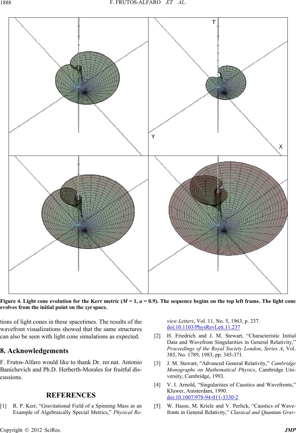

F. FRUTOS-ALFARO ET AL. 1888
Figure 4. Light cone evolution for the Kerr metric (M = 1, a = 0.9). The se quence begins on the top left frame. The light cone
evolves from the initial point on the xyt space.
tions of light cones in th ese spacetimes. The results of the
wavefront visualizations showed that the same structures
can also be seen with light cone simulations as expected.
8. Acknowledgements
F. Frutos-Alfaro would like to thank Dr. rer.nat. Antonio
Banichevich and Ph.D. Herberth-Morales for fruitful dis-
cussions.
REFERENCES
[1] R. P. Kerr, “Gravitational Field of a Spinning Mass as an
Example of Algebraically Special Metrics,” Physical Re-
view Letters, Vol. 11, No. 5, 1963, p. 237.
doi:10.1103/PhysRevLett.11.237
[2] H. Friedrich and J. M. Stewart, “Characteristic Initial
Data and Wavefront Singularities in General Relativity,”
Proceedings of the Royal Society London, Series A, Vol.
385, No. 1789, 1983, pp. 345-371.
[3] J. M. Stewart, “Advanced General Relativity,” Cambridge
Monographs on Mathematical Physics, Cambridge Uni-
versity, Cambridge, 1993.
[4] V. I. Arnold, “Singularities of Caustics and Wavefronts,”
Kluwer, Amsterdam, 1990.
doi:10.1007/978-94-011-3330-2
[5] W. Hasse, M. Kriele and V. Perlick, “Caustics of Wave-
front s in General Rel ativity,” Classical and Quantum Grav-

F. FRUTOS-ALFARO ET AL. 1889
ity, Vol. 13, No. 5, 1996, pp. 1161-1182.
doi:10.1088/0264-9381/13/5/027
[6] R. Low, “Stable Singularities of Wavefronts in General
Relativity,” Journal of Mathematical Physics, Vol. 36, No .
8, 1998, pp. 3332-3335. doi:10.1063/1.532257
[7] J. Ehlers and E. Newman, “The Theory of Caustics and
Wavefront Singularities with Physical Applications,” Jour-
nal of Mathematical Physics, Vol. 41, 2000, pp. 3344-
3378, arXiv:gr-qc/9906065. doi:10.1063/1.533316
[8] V. Perlick, “Gravitati onal Lensing from a Spacetime Per-
spective,” Living Reviews in Relativity, Vol. 7, No. 9,
2004, arXiv:1010.3416.
[9] K. P. Rauch and R. Blandford, “Optical Caustics in a
Kerr Spacetime and the Origin of Rapid X-Ray Variabil-
ity in Active Galactic Nuclei,” The Astrophysical Journal,
Vol. 421, No. 1, 1994, pp. 46-68. doi:10.1086/173625
[10] F. Grave, “Visualization of Gravitational Collapse and
Wavefronts in the General Relativity Theory, Diplomar-
beit,” Master Thesis, Eberhard Karls Universität Tübin-
gen, Tübingen, 2004.
[11] M. Sereno and F. De Luca, “Primary Caustics and Critical
Points behind a Kerr Black Hole,” Physical Review D,
Vol. 78, No. 2, 2008, Article ID: 023008, arXiv: astro-
ph/0710.5923.
[12] V. Bozza, “Optical Caustics of Kerr Spacetime: The Full
Structure,” Physical Review D, Vol. 78, No. 6, 2008, Ar-
ticle ID: 063014, arXiv:gr-qc/0806.4102.
[13] R. D. Blandford and R. Narayan, “Cosmological Applica-
tions of Gravitational Lensing,” Annual Review of As-
tronomy and Astrophysics, Vol. 30, 1992, pp. 311-358.
doi:10.1146/annurev.aa.30.090192.001523
[14] P. Schneider, J. Ehlers and E. E. Falco, “Gravitational
Lenses,” Springer, Berlin, 1992.
doi:10.1007/978-1-4612-2756-4
[15] H. Ohanian and R. Ruffini, “Gravitation and Spacetime,”
W. W. Norton & Company, New York, 1994.
[16] A. O. Petters, “Arnold’s Singularity Theory and Gravita-
tional Lensing,” Journal of Mathematical Physics, Vol.
34, No. 8, 1993, pp. 3555-3581. doi:10.1063/1.530045
[17] A. O. Petters, H. Levine and J. Wambsganss, “Singularity
The o r y a n d Gra vi t a t i o nal L ensin g,” S p ring e r , B e r l in, 2001.
doi:10.1007/978-1-4612-0145-8
[18] S. Frittelli and A. O. Petters. “Wave Fronts, Caustic
Sheets, and Caustic Surfing in Gravitational Lensing,”
Journal of Mathematical Physics, Vol. 43, No. 11, 2002,
pp. 5578-5611, arXiv:astro-ph/0208135.
doi:10.1063/1.1511790
[19] G. F. R. Ellis, B. A. Bassett and P. K. S. Dunsby, “Lens-
ing and Caustic Effects on Cosmological Distances,”
Classical and Quantum Gravity, Vol. 15, No. 8, 1998, pp.
2345-2361, arXiv:gr-qc/9801092v1.
doi:10.1088/0264-9381/15/8/015
[20] F. Grave, F. Frutos-Alfaro, T. Müller and D. Adis, “JWFront
in the Eleventh Marcel Grossmann Meeting: On Recent
Developments in Theoretical and Experimental General
Relativity,” In: H. Kleinert and R. T. Jantzen, Eds.,
Gravitation and Relativistic Field Theories, Proceedings
of the MG11 Meeting, World Scientific Publishing Com-
pany, London, 2008.
[21] R. d’Inverno, “Introducing Einstein’s Relativity,” Oxford
University Press, Oxford, 1992.
[22] C. W. Misner, K. S. Thorne and J. A. Wheeler, “Gravita-
tion,” Freeman, San Francisco, 1973.
[23] J. M. Bardeen, W. H. Press and S. A. Teukolsky, “Rotat-
ing Black Holes: Locally Nonrotating Frames, Energy
Extraction, and Scalar Synchrotron Radiation,” The As-
trophysical Journal, Vol. 178, 1972, pp. 347-369.
doi:10.1086/151796
[24] A. C. Hearn, “REDUCE (User’s and Contributed Pack-
ages Manual),” Konrad-Zuse-Zentrum für Information-
stechnik, Berlin, 1999.
[25] O. Semerák, “Spinning Test Particles in a Kerr Field-I,”
Monthly Notices of Royal Astronomical Society, Vol. 308,
No. 3, 1999, pp. 863-875.
doi:10.1046/j.1365-8711.1999.02754.x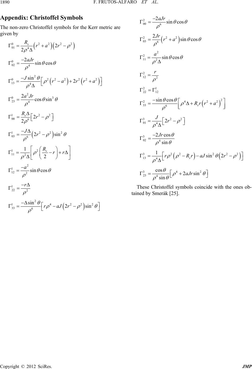

F. FRUTOS-ALFARO ET AL. 1890
Appendix: Christoffel Symbols
The non-zero Christoffel symbols for the Kerr metric are
given by
 
222
2r
02
01 4
2
s
Rra


 

0
02 2
4sin cos
aJr






2
022
13 4
sin 2 Jra 


 


2222
rra



2
03
cos sin
r
23 4
2aJ




122
62
Rr
00 2
s


  


1222
2sin
Jr
03 6



 

12
1
2
s
Rrr



 
 


11 2
 
2
1
12 2sin c
aos





1
22 2
r


 

2
14222
33 6
sin 2sinraJr 



 
 

2
00 6
2sin cos aJr






222
03 6
2sin cos Jr ra



 
2
2
11 2sin cos
a



 
2
12 2
r


21
22 12



2
2422
33 6
sin cos
s
Rr ra











322
01 42
Jr








3
02 4
2cos
sin
Jr





 
322222
13 4
1sin 2
s
rRraJr  







342
23 4
cos 2sin
sin aJr









These Christoffel symbols coincide with the ones ob-
tained by Smerák [25].
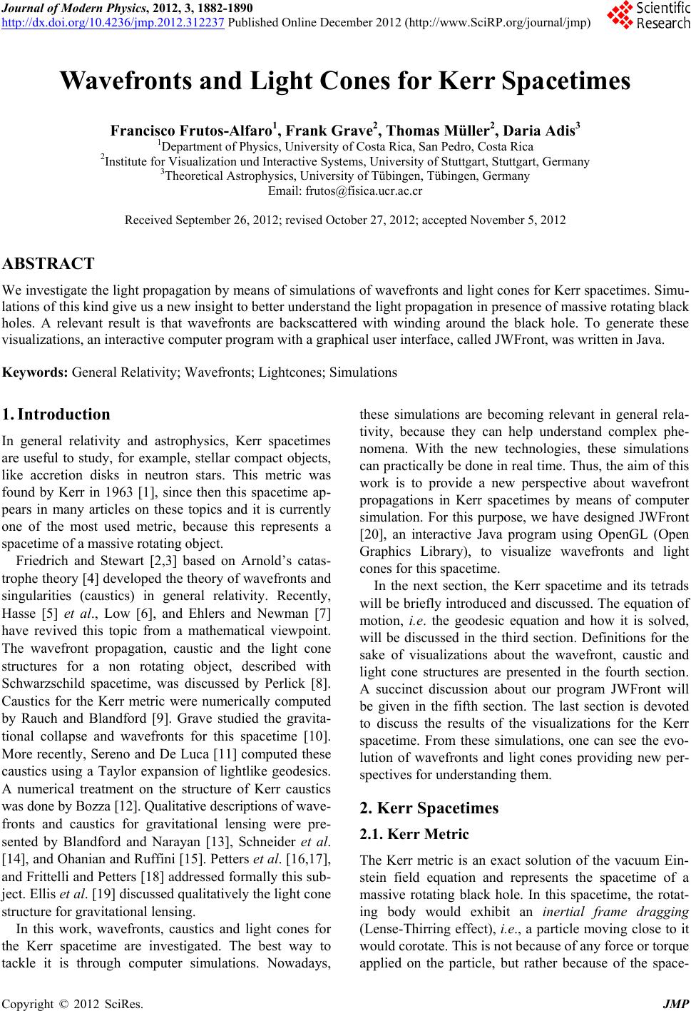