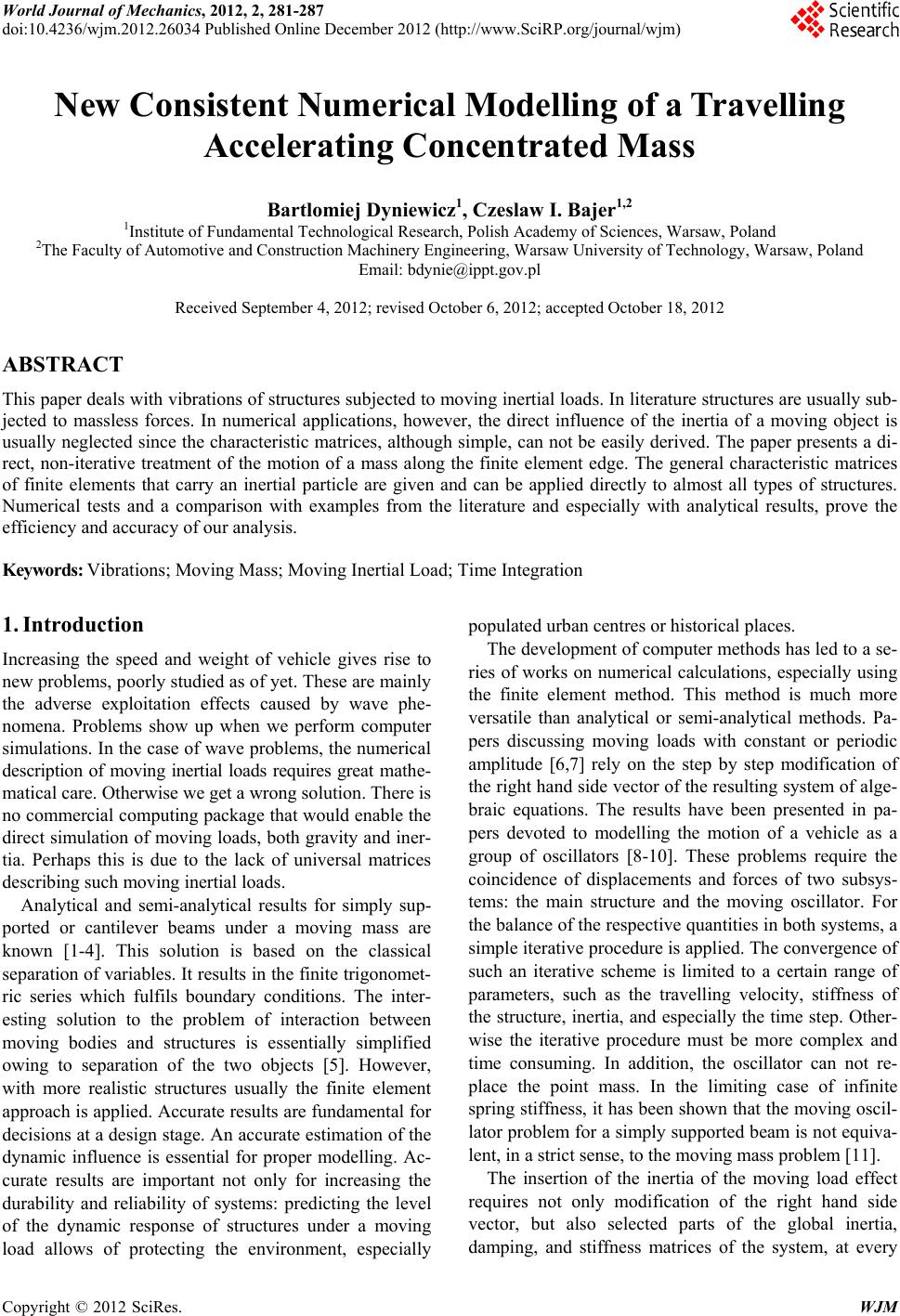
World Journal of Mechanics, 2012, 2, 281-287
doi:10.4236/wjm.2012.26034 Published Online December 2012 (http://www.SciRP.org/journal/wjm)
New Consistent Numerical Modelling of a Travelling
Accelerating Concentrated Mass
Bartlomiej Dyniewicz1, Czeslaw I. Bajer1,2
1Institute of Fundamental Technological Research, Polish Academy of Sciences, Warsaw, Poland
2The Faculty of Automotive and Construction Machinery Engineering, Warsaw University of Technology, Warsaw, Poland
Received September 4, 2012; revised October 6, 2012; accepted October 18, 2012
ABSTRACT
This paper deals with vibrations of structures subjected to moving inertial loads. In literature structures are usually sub-
jected to massless forces. In numerical applications, however, the direct influence of the inertia of a moving object is
usually neglected since the characteristic matrices, although simple, can not be easily derived. The paper presents a di-
rect, non-iterative treatment of the motion of a mass along the finite element edge. The general characteristic matrices
of finite elements that carry an inertial particle are given and can be applied directly to almost all types of structures.
Numerical tests and a comparison with examples from the literature and especially with analytical results, prove the
efficiency and accuracy of our analysis.
Keywords: Vibrations; Moving Mass; Moving Inertial Load; Time Integration
1. Introduction
Increasing the speed and weight of vehicle gives rise to
new problems, poorly studied as of yet. These are mainly
the adverse exploitation effects caused by wave phe-
nomena. Problems show up when we perform computer
simulations. In the case of wave problems, the numerical
description of moving inertial loads requires great mathe-
matical care. Otherwise we get a wrong solution. There is
no commercial computing package that would enable the
direct simulation of moving loads, both gravity and iner-
tia. Perhaps this is due to the lack of universal matrices
describing such moving inertial loads.
Analytical and semi-analytical results for simply sup-
ported or cantilever beams under a moving mass are
known [1-4]. This solution is based on the classical
separation of variables. It results in the finite trigonomet-
ric series which fulfils boundary conditions. The inter-
esting solution to the problem of interaction between
moving bodies and structures is essentially simplified
owing to separation of the two objects [5]. However,
with more realistic structures usually the finite element
approach is applied. Accurate results are fundamental for
decisions at a design stage. An accurate estimation of the
dynamic influence is essential for proper modelling. Ac-
curate results are important not only for increasing the
durability and reliability of systems: predicting the level
of the dynamic response of structures under a moving
load allows of protecting the environment, especially
populated urban centres or historical places.
The development of computer methods has led to a se-
ries of works on numerical calculations, especially using
the finite element method. This method is much more
versatile than analytical or semi-analytical methods. Pa-
pers discussing moving loads with constant or periodic
amplitude [6,7] rely on the step by step modification of
the right hand side vector of the resulting system of alge-
braic equations. The results have been presented in pa-
pers devoted to modelling the motion of a vehicle as a
group of oscillators [8-10]. These problems require the
coincidence of displacements and forces of two subsys-
tems: the main structure and the moving oscillator. For
the balance of the respective quantities in both systems, a
simple iterative procedure is applied. The convergence of
such an iterative scheme is limited to a certain range of
parameters, such as the travelling velocity, stiffness of
the structure, inertia, and especially the time step. Other-
wise the iterative procedure must be more complex and
time consuming. In addition, the oscillator can not re-
place the point mass. In the limiting case of infinite
spring stiffness, it has been shown that the moving oscil-
lator problem for a simply supported beam is not equiva-
lent, in a strict sense, to the moving mass problem [11].
The insertion of the inertia of the moving load effect
requires not only modification of the right hand side
vector, but also selected parts of the global inertia,
damping, and stiffness matrices of the system, at every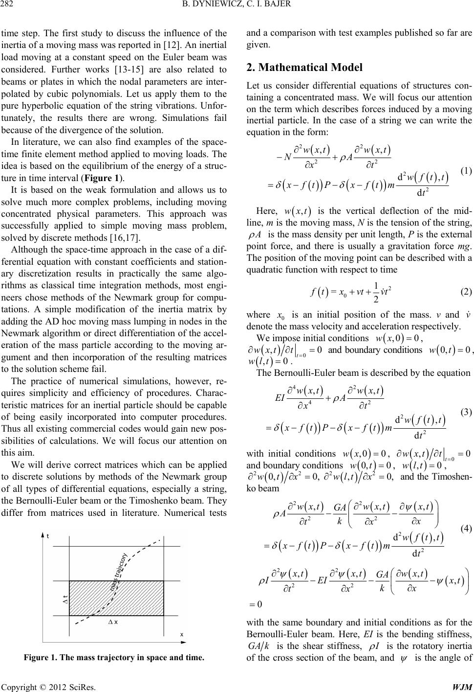

B. DYNIEWICZ, C. I. BAJER
282
time step. The first study to discuss the influence of the
inertia of a moving mass was reported in [12]. An inertial
load moving at a constant speed on the Euler beam was
considered. Further works [13-15] are also related to
beams or plates in which the nodal parameters are inter-
polated by cubic polynomials. Let us apply them to the
pure hyperbolic equation of the string vibrations. Unfor-
tunately, the results there are wrong. Simulations fail
because of the divergence of the solution.
In literature, we can also find examples of the space-
time finite element method applied to moving loads. The
idea is based on the equilibrium of the energy of a struc-
ture in time interval (Figure 1).
It is based on the weak formulation and allows us to
solve much more complex problems, including moving
concentrated physical parameters. This approach was
successfully applied to simple moving mass problem,
solved by discrete methods [16,17].
Although the space-time approach in the case of a dif-
ferential equation with constant coefficients and station-
ary discretization results in practically the same algo-
rithms as classical time integration methods, most engi-
neers chose methods of the Newmark group for compu-
tations. A simple modification of the inertia matrix by
adding the AD hoc moving mass lumping in nodes in the
Newmark algorithm or direct differentiation of the accel-
eration of the mass particle according to the moving ar-
gument and then incorporation of the resulting matrices
to the solution scheme fail.
The practice of numerical simulations, however, re-
quires simplicity and efficiency of procedures. Charac-
teristic matrices for an inertial particle should be capable
of being easily incorporated into computer procedures.
Thus all existing commercial codes would gain new pos-
sibilities of calculations. We will focus our attention on
this aim.
We will derive correct matrices which can be applied
to discrete solutions by methods of the Newmark group
of all types of differential equations, especially a string,
the Bernoulli-Euler beam or the Timoshenko beam. They
differ from matrices used in literature. Numerical tests
Figure 1. The mass trajectory in space and time.
and a comparison with test examples published so far are
given.
2. Mathematical Model
Let us consider differential equations of structures con-
taining a concentrated mass. We will focus our attention
on the term which describes forces induced by a moving
inertial particle. In the case of a string we can write the
equation in the form:




   


22
22
2
2
,,
d,
d
wxtwxt
NA
xt
wft t
xftP xftmt





 
(1)
Here,


,wxt is the vertical deflection of the mid-
line, m is the moving mass, N is the tension of the string,
A

is the mass density per unit length, P is the external
point force, and there is usually a gravitation force mg.
The position of the moving point can be described with a
quadratic function with respect to time

2
0
1
=2
f
tx vtvt (2)
where 0
x
is an initial position of the mass. v and v

denote the mass velocity and acceleration respectively.
We impose initial conditions

,0 0wx ,


0
,0
t
wxtt

 and boundary conditions


0, 0wt

,


,0wlt

.
The Bernoulli-Euler beam is described by the equation


   
 
42
42
2
2
,,
d,
d
wxtwxt
EI A
xt
wft t
xftP xftmt





 
(3)
with initial conditions


,0 0wx ,

0
,0
t
wxtt 
and boundary conditions

0, 0wt,

,0wlt

,




2222
0, 0,, 0,wt xwlt x

  and the Timoshen-
ko beam

 
   
 
22
22
2
2
,,,
d,
d
w xtw xtxt
GA
Akx
tx
wft t
xftP xftmt








 

 
(4)



 
22
22
,, ,
,
0
xtxtw xt
GA
I
EIx t
kx tx


  
 

 


with the same boundary and initial conditions as for the
Bernoulli-Euler beam. Here, EI is the bending stiffness,
GAk is the shear stiffness,
I

is the rotatory inertia
of the cross section of the beam, and

is the angle of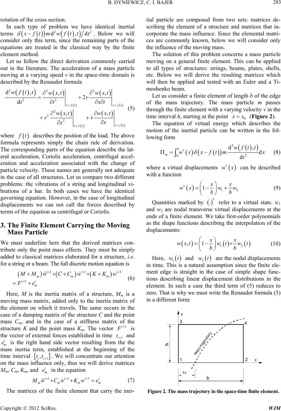

B. DYNIEWICZ, C. I. BAJER
283
rotation of the cross section.
In each type of problem we have identical inertial
terms
   
22
d,d
x
ftmwft tt  . Below we will
consider only this term, since the remaining parts of the
equations are treated in the classical way by the finite
element method.
Let us follow the direct derivation commonly carried
out in the literature. The acceleration of a mass particle
moving at a varying speed v in the space-time domain is
described by the Renaudot formula












222
22
2
2
2
d, ,,
2
d
,,
xft xft
x
ft
xft
wft twxtwxt
vxt
tt
wxt wxt
vv
x x











(5)
where

f
t describes the position of the load. The above
formula represents simply the chain rule of derivation.
The corresponding parts of the equation describe the lat-
eral acceleration, Coriolis acceleration, centrifugal accel-
eration and acceleration associated with the change of
particle velocity. These names are generally not adequate
in the case of all structures. Let us compare two different
problems: the vibrations of a string and longitudinal vi-
brations of a bar. In both cases we have the identical
governing equation. However, in the case of longitudinal
displacements we can not call the forces described by
terms of the equation as centrifugal or Coriolis.
3. The Finite Element Carrying the Moving
Mass Particle
We must underline here that the derived matrices con-
tribute only the point mass effects. They must be simply
added to classical matrices elaborated for a structure, i.e.
for a string or a beam. The full discrete motion equation is






11 1
1
ii i
mm m
ii
m
M
Mw CCwKKw
Fe
 



 
(6)
Here, M is the inertia matrix of a structure, Mm is a
moving mass matrix, added only to the inertia matrix of
the element on which it travels. The same occurs in the
case of a damping matrix of the structure C and the point
mass Cm, and in the case of a stiffness matrix of the
structure K and the point mass Km. The vector 1i
F

is
the vector of external forces established in time 1i
t

and
i
m
e is the right hand side vector resulting from the the
mass inertia term, established at the beginning of the
time interval


1
,
ii
tt
. We will concentrate our attention
on the mass influence only, thus we will derive matrices
Mm, Cm, Km, and i
m
e in the equation
11 1ii ii
mm mm
M
wCwKwe
 
 
  (7)
The matrices of the finite element that carry the iner-
tial particle are composed from two sets: matrices de-
scribing the element of a structure and matrices that in-
corporate the mass influence. Since the elemental matri-
ces are commonly known, below we will consider only
the influence of the moving mass.
The solution of this problem concerns a mass particle
moving on a general finite element. This can be applied
to all types of structures: strings, beams, plates, shells,
etc. Below we will derive the resulting matrices which
will then be applied and tested with an Euler and a Ti-
moshenko beam.
Let us consider a finite element of length b of the edge
of the mass trajectory. The mass particle m passes
through the finite element with a varying velocity v in the
time interval h, starting at the point 0
x
x (Figure 2).
The equation of virtual energy which describes the
motion of the inertial particle can be written in the fol-
lowing form
  
 
2
2
0
d,
d
d
b
m
wft t
wxxftmx
t


 
 (8)
where a virtual displacements


wx
 can be described
with a function

12
1xx wxw w
bb

 

 (9)
Quantities marked by

*
. refer to a virtual state. w1
and w2 are nodal transverse virtual displacements at the
ends of a finite element. We take first-order polynomials
as the shape functions describing the interpolation of the
displacements:
  
12
,1
xx
wxtw twt
bb

 

 (10)
Here,


1
wt and


2
wt are the nodal displacements
in time. This is a natural assumption since the finite ele-
ment edge is straight in the case of simple shape func-
tions describing linear displacement distributions in the
element. In such a case the third term of (5) reduces to
zero. That is why we must write the Renaudot formula (5)
in a different form:
x
0
Figure 2. The mass trajectory in the space-time finite element.

B. DYNIEWICZ, C. I. BAJER
284
 








2
2
22
2
d,
d
,,
,,
d
d
xft xft
xft xft
wft t
t
wxt wxt
vxt
t
wxt wxt
vv
xtx




 








(11)
The fourth term of (11) is developed in a Taylor series
in terms of the time increment th









,
,,
d1
d
,
d
d
th
xft
t
t
xft xft
th
xft
wxt
x
wxtwxth
xtx
wxth
tx


















 

 














(12)
Upper indices indicate the time in which the respective
terms are defined. We assume the backward difference
formula (

=1). In this case we have






,
d
d
,,
11
th
xft
th t
xft xft
wxt
tx
wxt wxt
hx hx






















(13)
According to Equations (2), (10) and (13), Equation (11)
is given by the difference formula
 
2
2
11111
12121
111
21 212
d
d
1iiiii
iiiii
w
t
fhfh vvv
wwwww
bbbbb
vv v vv
wwwww
bbhbhbhbh







  

 

(14)
The upper index denotes time layer. The energy (8),
with respect to (9) and (14) can be written in quadratic
form, which, after a classical minimization, results in the
matrix Equation (7), where
 

2
2
11
1
m
Mm

 






(15)

11
m
mv
Cb



 



(16)

11
m
mv
Kv
bh


 







 (17)
and

 

21
21
1
m
ww
mv
eww
bh









 (18)
with coefficient 2
0
1,0 1
2
xvhvh b



 


.
Here,

is a parameter which defines the position of
the mass in the element at the beginning of the time in-
crement.
This determines the position of the mass at time th

,
related to the finite element length b. The different terms
describe the transverse inertia force related to the vertical
acceleration, the Coriolis force, and the centrifugal force.
The matrix factors Mm, Cm, and Km can be called the
mass, damping, and stiffness matrices. The last term m e
describes the nodal forces at the beginning of the time
interval


,
ii
tt t

. We must emphasize here that the
matrices (15)-(17) and the vector (18) contribute only the
moving inertial particle effect. The matrices of the mass
influence in a finite element of a structure must be added
to the global system of equations. We notice that the ma-
trices (15)-(17) differ from the matrices that cause the
divergence of the solution in the case of direct differen-
tiation of (5)1.
4. Numerical Results
The scheme of computations is given in Figure 3:
The finite element is subjected at a mid-point to the
force and the inertia parameter, i.e. the concentrated mass.
The force vector, usually placed at the right hand side of
the resulting system of algebraic equations, is simply
distributed over neighbouring nodes (bending moments
in the case of a beam must be considered in nodes as
Figure 3. Theoretical scheme of the problem and the sche me
assumed for computations.
1The matrices that result in the divergence:
2
2
(1 )(1 )(1 )1
2
==
(1 )
mm
mv
MmC b



 

  



  

2
0
1
(1) 12
==,0<1.
m
xvh vh
mv
Kbb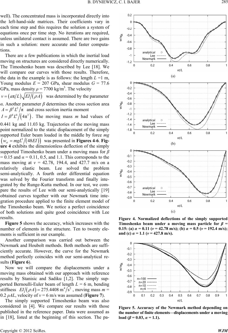




  






B. DYNIEWICZ, C. I. BAJER
285
well). The concentrated mass is incorporated directly into
the left-hand-side matrices. Their coefficients vary in
each time step and this requires the solution a system of
equations once per time step. No iterations are required,
unless unilateral contact is assumed. There are two gains
in such a solution: more accurate and faster computa-
tions.
There are a few publications in which the inertial load
moving on structures are considered directly numerically.
The Timoshenko beam was described by Lee [18]. We
will compare our curves with those results. Therefore,
the data in the example is as follows: the length L =1 m,
Young modulus E = 207 GPa, shear modulus G = 77.6
GPa, mass density ρ = 7700 kg/m3. The velocity

πvaLEIA   was determined by the parameter
α. Another parameter β determines the cross section area
22πAL
  and cross section inertia moment

44 3
4πIL  . The moving mass m had values of
0.441 kg and 11.03 kg. Trajectories of the moving mass
point normalized to the static displacement of the simply
supported Euler beam loaded in the middle by force mg


348
st
wmgL EI was presented in Figures 4-6. Fig-
ure 4 exhibits the dimensionless deflection of the simply
supported Timoshenko beam under a moving mass for β
= 0.15 and α = 0.11, 0.5, and 1.1. This corresponds to the
mass moving at v = 42.78, 194.4, and 427.7 m/s on a
relatively elastic beam. Lee solved the problem
semi-analytically. A fourth order differential equation
was solved by the Fourier transform and finally inte-
grated by the Runge-Kutta method. In our test, we com-
pare the results of Lee with our semi-analytically [19]
obtained curves together with our Newmark time inte-
gration procedure applied to the finite element model of
the Timoshenko beam. We notice a perfect coincidence
of both solutions and quite good coincidence with Lee
results.
Figure 5 shows the accuracy, which increases with the
number of elements in the structure. Ten to twenty ele-
ments is sufficient in our example.
Another comparison was carried out between the
Newmark and Houbolt methods. Both methods are suffi-
ciently accurate. However, the curve for the Newmark
method perfectly coincides with our semi-analytical re-
sults (Figure 6).
Now we will compare the displacements under a
moving mass obtained with our approach with reference
results by Stanisic and Sadiku [1,2]. The simply sup-
ported Bernoulli-Euler beam of length L = 6 m, bending
stiffness

42
275.4408 msEI A  , moving mass m =
0.2 ρAL, velocity of v = 6 m/s was assumed (Figure 7).
The simply supported Timoshenko beam was also
considered in [4]. We compare our results with those
published in the reference paper. Data were assumed as
in [18], listed at the beginning of this section. The pa-
(a)
(b)
(c)
Figure 4. Normalized deflections of the simply supported
Timoshenko beam under a moving mass particle for β =
0.15: (a) α = 0.11 (v = 42.78 m/s); (b) α = 0.5 (v = 192.4 m/s);
and (c) α = 1.1 (v = 427.8 m/s).
Figure 5. Accuracy of the Newmark method depending on
the number of finite elements—displacements under a moving
load (β = 0.03, α = 1.1).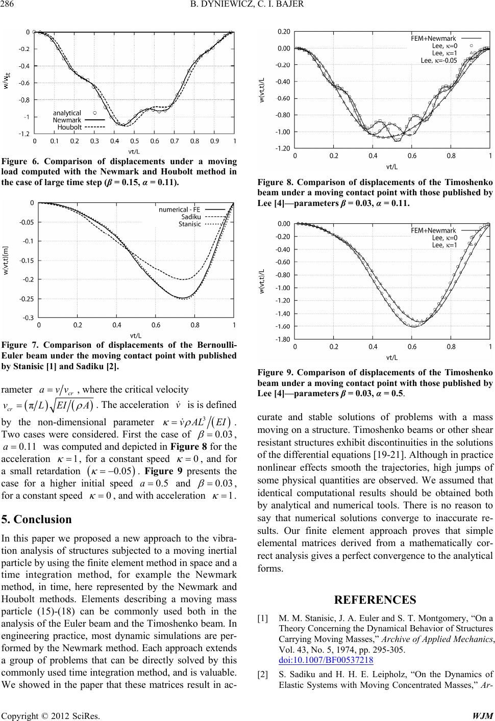

B. DYNIEWICZ, C. I. BAJER
286
Figure 6. Comparison of displacements under a moving
load computed with the Newmark and Houbolt method in
the case of large time step (β = 0.15, α = 0.11).
Figure 7. Comparison of displacements of the Bernoulli-
Euler beam under the moving contact point with published
by Stanisic [1] and Sadiku [2].
rameter cr avv, where the critical velocity
 
π
cr
vLEIA

. The acceleration v
 is is defined
by the non-dimensional parameter


3
vAL EI  .
Two cases were considered. First the case of 0.03


,
0.11a was computed and depicted in Figure 8 for the
acceleration 1  , for a constant speed 0  , and for
a small retardation

0.05   . Figure 9 presents the
case for a higher initial speed 0.5a and 0.03


,
for a constant speed 0  , and with acceleration 1


.
5. Conclusion
In this paper we proposed a new approach to the vibra-
tion analysis of structures subjected to a moving inertial
particle by using the finite element method in space and a
time integration method, for example the Newmark
method, in time, here represented by the Newmark and
Houbolt methods. Elements describing a moving mass
particle (15)-(18) can be commonly used both in the
analysis of the Euler beam and the Timoshenko beam. In
engineering practice, most dynamic simulations are per-
formed by the Newmark method. Each approach extends
a group of problems that can be directly solved by this
commonly used time integration method, and is valuable.
We showed in the paper that these matrices result in ac-
Figure 8. Comparison of displacements of the Timoshenko
beam under a moving contact point with those published by
Lee [4]—parameters β = 0.03, α = 0.11.
Figure 9. Comparison of displacements of the Timoshenko
beam under a moving contact point with those published by
Lee [4]—parameters β = 0.03, α = 0.5.
curate and stable solutions of problems with a mass
moving on a structure. Timoshenko beams or other shear
resistant structures exhibit discontinuities in the solutions
of the differential equations [19-21]. Although in practice
nonlinear effects smooth the trajectories, high jumps of
some physical quantities are observed. We assumed that
identical computational results should be obtained both
by analytical and numerical tools. There is no reason to
say that numerical solutions converge to inaccurate re-
sults. Our finite element approach proves that simple
elemental matrices derived from a mathematically cor-
rect analysis gives a perfect convergence to the analytical
forms.
REFERENCES
[1] M. M. Stanisic, J. A. Euler and S. T. Montgomery, “On a
Theory Concerning the Dynamical Behavior of Structures
Carrying Moving Masses,” Archive of Applied Mechanics,
Vol. 43, No. 5, 1974, pp. 295-305.
doi:10.1007/BF00537218
[2] S. Sadiku and H. H. E. Leipholz, “On the Dynamics of
Elastic Systems with Moving Concentrated Masses,” Ar-

B. DYNIEWICZ, C. I. BAJER
287
chive of Applied Mechanics, Vol. 57, No. 3, 1987, pp.
223-242.
[3] H. P. Lee, “On the Dynamic Behaviour of a Beam with an
Accelerating Mass,” Archive of Applied Mechanics, Vol.
65, No. 8, 1995, pp. 564-571. doi:10.1007/BF00789097
[4] H. P. Lee, “Transverse Vibration of a Timoshenko Beam
Acted on by an Accelerating Mass,” Applied Acoustics,
Vol. 47, No. 4, 1996, pp. 319-330.
doi:10.1016/0003-682X(95)00067-J
[5] V. A. Krysko, J. Awrejcewicz, A. N. Kutsemako and K.
Broughan, “Interaction between Flexible Shells (Plates)
and a Moving Lumped Body,” Communications in Non-
linear Science and Numerical Simulation, Vol. 11, No. 1,
2006, pp. 13-43. doi:10.1016/j.cnsns.2004.06.006
[6] J. J. Wu, A. R. Whittaker and M. P. Cartmell, “The Use
of Finite Element Techniques for Calculating the Dy-
namic Response of Structures to Moving Loads,” Com-
puters and Structures, Vol. 78, No. 6, 2000, pp. 789-799.
doi:10.1016/S0045-7949(00)00055-9
[7] P. Lou, G. Dai and Q. Zeng, “Dynamic Analysis of a
Timoshenko Beam Subjected to Moving Concentrated
Forces Using the Finite Element Method,” Shock and Vi-
bration, Vol. 14, No. 6, 2007, pp. 459-468.
[8] J. Hino, T. Yoshimura, K. Konishi and N. Ananthanara-
yana, “A Finite Element Prediction of the Vibration of a
Bridge Subjected to a Moving Vehicle Load,” Journal of
Sound and Vibration, Vol. 96, No. 1, 1984, pp. 45-53.
doi:10.1016/0022-460X(84)90593-5
[9] Y. H. Lin and M. W. Tretheway, “Finite Element Analy-
sis of Elastic Beams Subjected to Moving Dynamic
Loads,” Journal of Sound and Vibration, Vol. 136, No. 2,
1990, pp. 323-342. doi:10.1016/0022-460X(90)90860-3
[10] Y. S. Cheng, F. T. K. Au and Y. K. Cheung, “Vibration
of Railway Bridges under a Moving Train by Using
Bridge-Track-Vehicle Element,” Engineering Structures,
Vol. 23, No. 12, 2001, pp. 1597-1606.
doi:10.1016/S0141-0296(01)00058-X
[11] A. V. Pesterev, L. A. Bergman, C. A. Tan, T.-C. Tsao and
B. Yang, “On Asymptotics of the Solution of the Moving
Oscillator Problem,” Journal of Sound and Vibration, Vol.
260, No. 3, 2003, pp. 519-536.
doi:10.1016/S0022-460X(02)00953-7
[12] D. M. Yoshida and W. Weaver, “Finite-Element Analysis
of Beams and Plates with Moving Loads,” Journal of the
International Association Bridge and Structural Engi-
neering, Vol. 31, No. 1, 1971, pp. 179-195.
[13] F. V. Filho, “Finite Element Analysis of Structures under
Moving Loads,” The Shock and Vibration Digest, Vol. 10,
No. 8, 1978, pp. 27-35.
doi:10.1177/058310247801000803
[14] A. O. Cifuentes, “Dynamic Response of a Beam Excited
by a Moving Mass,” Finite Elements in Analysis and De-
sign, Vol. 5, No. 3, 1989, pp. 237-246.
doi:10.1016/0168-874X(89)90046-2
[15] J. R. Rieker, Y. H. Lin and M. W. Trethewey, “Discreti-
zation Considerations in Moving Load Finite Element
Beam Models,” Finite Elements in Analysis and Design,
Vol. 21, No. 3, 1996, pp. 129-144.
doi:10.1016/0168-874X(95)00029-S
[16] C. I. Bajer and B. Dyniewicz, “Space-Time Approach to
Numerical Analysis of a String with a Moving Mass,” In-
ternational Journal for Numerical Methods in Engineer-
ing, Vol. 76, No. 10, 2008, pp. 1528-1543.
[17] C. I. Bajer and B. Dyniewicz, “Virtual Functions of the
Space-Time Finite Element Method in Moving Mass
Problems,” Computers and Structures, Vol. 87, No. 7-8,
2009, pp. 444-455. doi:10.1016/j.compstruc.2009.01.007
[18] H. P. Lee, “The Dynamic Response of a Timoshenko
Beam Subjected to a Moving Mass,” Journal of Sound
Vibration, Vol. 198, No. 2, 1996, pp. 249-256.
doi:10.1006/jsvi.1996.0567
[19] B. Dyniewicz and C. I. Bajer, “New Feature of the Solu-
tion of a Timoshenko Beam Carrying the Moving Mass
Particle,” Archive of Mechanics, Vol. 62, No. 5, 2010, pp.
327-341.
[20] B. Dyniewicz and C. I. Bajer, “Paradox of the Particle’s
Trajectory Moving on a String,” Archive Applied Me-
chanics, Vol. 79, No. 3, 2009, pp. 213-223.
doi:10.1007/s00419-008-0222-9
[21] B. Dyniewicz and C. I. Bajer, “Discontinuous Trajectory
of the Mass Particle Moving on a String or a Beam,”
Machine Dynamics Problems, Vol. 31, No. 2, 2007, pp.
66-79.