Open Journal of Applied Sciences, 2012, 2, 257-266
doi:10.4236/ojapps.2012.24038 Published Online December 2012 (http://www.SciRP.org/journal/ojapps)
Evaluation Strategies for Coupled GC-IMS Measurement
including the Systematic Use of Parametrized ANN
Training Data
Artur Scheinemann1, Stefanie Sielemann2, Jӧrg Walter2, Theodor Doll1
1Institute of Physics, Johannes Gutenberg-University Mainz, Mainz, Germany
2Gesellschaft für Analytische Sensorsysteme mbH G.A.S., Dortmund, Germany
Received August 24, 2012; revised September 26, 2012; accepted October 8, 2012
ABSTRACT
Data evaluation strategies for the novel coupled MCC-IMS sensory system are developed. Mayor attention to the plau-
sibility of applied procedures and the feasibility of automation was paid. Three stages of extraction levels with increas-
ing data reduction are presented for several fields of application. According to suitable extraction levels, real data were
tested on various structures of artificial neural networks (ANN) with the result, that the computational levels must still
be chosen by expertise, but subsequent processing and training can be fully automated. For the training of larger net-
works a method of automated generation of secondary training data is presented which exceeds the quality of previous
noise models by far. It is concluded that the combination of MCC-IMS as measuring instrument and ANNs as evalua-
tion technique have high potential for industrial use in process monitoring.
Keywords: Gas Chromatography; Ion Mobility Spectrometry; GC-IMS; MCC-IMS; Artificial Neural Network;
Measurement Evaluation
1. Introduction
Ion Mobility Spectrometry (IMS [1]) and Gas Chroma-
tography (GC [2]) have been well established measuring
technologies for several decades. However their coupling
into a combined measuring technology (GC-IMS) is rela-
tively new [3,4]. Though this method is very promising
in terms of sensitivity and accuracy, all evaluation tools
have to be developed from the very beginning. Several
attempts have been made to find an analytical approach
for the description of GC-IMS spectra in order to auto-
mate the evaluation of these measurements, only little
progress was gained [5,6]. Due to their 2-dimensional
nature GC-IMS measurements contain great quantities of
data, which, depending on the measurement setup, may
contain up toor evendata points.
6
10 7 10
2. Experimental Details
2.1. Measuring Principle and Resulting
Properties of the Measurements
The GC-IMS is a system that measures 2 different pro-
perties independent from each other [7-9]. While the GC
column separates analytes depending on their ability to
adsorb and desorb on the inner column surface (see Fig-
ure 1), the IMS separates charged particles under the
influence of an electrical field depending on their drift
behavior in a carrier gas atmosphere. This can be seen in
Figure 2. Beginning at the moment of the analyte injec-
tion into the GC column the output of the GC column is
permanently analyzed by the IMS. At a given rate per
second the IMS is recording 1-dimensional spectra until
all fractions of the analyte have been eluted from the
column. The taken 1-dimensional spectra are combined
into one 2-dimensional spectrum with certain character-
istics as it can be seen in Figure 3.
The carrier gas is always present in the measurement
process and therefore is seen in all spectra. The accord-
ing peak in the spectrum is called RIP (Reactant Ion
Peak). The RIP is a constant feature of IMS spectra. The
ions which are analyzed by the IMS are ionized by a ra-
diation source in the reaction region of the IMS and then
pulled by an electrical field toward the detector. The time
from the opening of the gate, when the electric field
starts to pull the ions till they hit the detector and cause
an electric current is called the drift time of this particu-
lar ion sort. The ionized carrier gas (reactant ions) reacts
with the analyte sample when latter is eluted from the
GC into the IMS. Due to the reaction mechanism the
formation of analyte ions competes with the amount of

A. SCHEINEMANN ET AL. 258
reactant ions present in the reaction region. Hence the
detection of a peak at a given retention time
R
t reduces
the intensity of the RIP at the same
R
t(see Figure 3).
Since the radiation in the ionization region is constant,
the amount of produced ions is assumed to by nearly
constant and hence the amount of detected charged parti-
cles at the Faraday detector.
Thus a decreasing or even vanishing RIP intensity is
always the result of detected analytes forming a peak at
D
RIP and preserving the overall ion amount detected
at a given retention time
tt
R
t.
 
,max
1
dd
=,d
dd
tD
RDR
RR
QtIt tt
tt 
0 D
(1)
2.2. Available Measurement Data
Depending on the processing approach, the demanded
Figure 1. Schematic draft of the measurement technique
and the gas flow inside of a GC-IMS detector.
amount of measurement data to initialize a certain pro-
cessing algorithm can differ by orders of magnitude.
Here initialization means a first and one-time execution
of the algorithm code which sets the processing program
into the state where it can simply read an unknown
measurement sample and produce an appropriate output
to classify the unknown sample. Initialization can be the
storage of reference samples, the evaluation of reference
samples in order to adopt certain threshold parameters
which determine the classification process or the training
of an ANN. Furthermore any processing algorithm, once
initialized, needs to be evaluated with new data sets that
were not used before during the initialization.
The most simple case is the attempt to distinguish be-
tween two possible categories for example the breath of
people with and without some specific decease or the
detection of some specific contaminant in any food or be-
verage product.
Since every processing approach has to be evaluated
with really measured data it is important to have a dataset
of measurements big enough. Though the motto is, the
bigger the dataset the better for the evaluation, the analy-
sis in this work had to content itself to the dataset given
in Table 1. The measurements were carried out using the
FlavourSpec and GC-IMS by G.A.S. Both systems con-
sist of a combination of an IMS with a chromatographic
column for a better pre separation of volatile organic
compounds (VOCs) in complex mixtures. The essential
technical and physical data of the measuring devices are
essembled in Listing 1.
The involved interaction potentials between drift gas
and analyze particles are of enormous complexity. This is
especially the case with complex analyze particles as
MVOCs. There are no analytical models to predict the
appearance of a molecule or atom in the spectra just from
analyte
Figure 2. Schematic picture of the IMS and its parts.

A. SCHEINEMANN ET AL. 259
Table 1. Data sets for GC-IMS analysis tests.
Measurement
class Categories Measurements Measurements total
Cola 13 ≈10 130
Juice 18 ≈10 180
Rice 4 ≈5 20
Olive oil 3 ≈50 147
Breath diff.
candy flavors 3 ≈16 50
Meat 14 ≈5 70
-IMS Parameters
-- Drift length: 50 mm
-- Drift voltage: 2 kV
-- Electrical field strength: 400 V/cm
-Radioactive Ionisation source
-- Tritium 3H (-radiation

) 300 MBq
-- Radioactive half-life: 12.5 years
-Multi Capillary Column (MCC) Parameters
-- Film thickness: 0.2 μm
-- Column Lenght: 20 cm
-- Capillaries I.D. μm: 40
-- Number of capillaries: 1200
Listing 1. Technical Specs of used GC-IMS.
fundamental modeling using first principle physics. An-
other way to distinguish between different spectra would
therefore be of interest. In the following alternative ap-
proaches for evaluation and processing of GC-IMS spec-
tra are presented. The benefits of using them in Neural
Networks are discussed and results of classification tests
produced by them are presented.
One problem is to find a suitable and general evalua-
tion strategy which helps to determine from which cate-
gory a given measurement is. A successful strategy not
only has to yield stable classification rates on unseen
spectra/measurements, it furthermore needs to be general
enough to be applied to new classification problems
without cumbersome modifications.
3. Simple Metrics Evaluation
After inspecting the spectra of the breath measurements
(two measurements from two different flavors can be
seen in Figure 4) a quite simple and straight forward
approach gets obvious. It is to define a metrics on the
two dimensional spectra in order to determine a distance
between two spectra. One possible definition of this dis-
tance between two arbitrary spectra and


,

,
iRD
Rtt


R
D
M
tt is:


,max ,max
=1 =1
=,
=,
DD
DR
ii
tt
iRD RD
tt
dRM
Rtt Mtt


 ,
(2)
This method needs only one reference measurement
Figure 3. GC-IMS spectrum shown in perspective view with
the duality of RIP and Peak. This is an artificial illustration
intended to visualize basic principles of GC-IMS measure-
ments. It is therefore exaggerated and not completely con-
sistent since the smaller peaks should as well diminish the
RIP intensity. The properties of this spectrum are discussed
in the text.
Figure 4. Two different candy flavors taken from the breath
measurement. The spectra show obvious differences. Left:
Candy flavor 1; Right: Candy flavor 2 (see Table 2 for the
complete list of measurements).
i for every substance i that needs to be classified.
Any uncategorized measurement
R
M
would then be
evaluated against all references and the minimum
distance min of all distances i
would be
given as the most likely classification result for the un-
known measurement. Meaning that if min than
is the category where M most likely belongs to.
d

,RM
=k
d

=
i
d
dk
We find that only measurement categories with visible,
obvious differences like those in Figure 4 (like the
breath samples with different candy flavors as seen in
Figure 4) can be separated by this algorithm.
Since the simplest straight forward approach doesn’t
work and several attempts to align measurements ac-
cording to the RIP position failed to gain any improve-
ment, it is mandatory to get more insight into the meas-
uring principle.

A. SCHEINEMANN ET AL. 260
4. Profile Evaluation
4.1. Evaluation of RIP Profiles
Given the measuring characteristics explained in Section
2.1, one could use the RIP-shape for further analysis and
neglect the information given by the points with
>
D
RIP
tt. By doing so the magnitude of data points is
reduced from millions down to several hundreds. Figure
5 shows an exemplary extraction of a RIP-Profile along
the retention time axis. At fixed drift time (which is the
drift time of the RIP peak) the intensity values along the
retention time axis are extracted and combined to one
profile. This process can be automated because the RIP
can be easily found in every GC-IMS measurement. This
approach, though being simplifying, allows the use of
Artificial Neural Networks (ANNs) for the evaluation
and classification of measured spectra. The use of ANNs
seems even imperative. As can bee seen in Figure 6 from
the overlaid different spectra, it is not possible to define
discrimination levels for the signals to distinguish be-
tween different measurements without multi-feature ana-
lysis, for which ANN are well suited if training data are
sufficient.
4.2. Evaluation of Drift Profiles
The extraction of the RIP profiles looses a lot of infor-
mation that is enclosed in the drift axis. A similar ap-
proach would be to extract a profile along the drift time
axis and to lose information that is enclosed in the reten-
tion time axis. Since there is no exceptional point along
the retention time axis like the RIP is on the drift time
axis one has to find another extraction formalism differ-
ing from the RIP profile extraction. Two possible ways
to obtain a drift profile

D
Dt are:
 
,max
=1
=
R
R
t
,
D
DR
t
DtIt t
 (3)
or





,,
=max ,0,
DRIPD RRR
DtIt ttt


max


(4)
Equation (3) is nothing else then just a simple IMS
measurement, since all information that was gained dur-
ing the separation process of the GC column was now
again summed up as if it was never separated. Since
Equation (4) is a projection and doesn’t integrate all in-
formation along the retention time axis for every point in
our drift spectrum this evaluation formalism was used.
4.3. Virtual Measurements
Depending on the setup, the RIP-Profiles contain from
up todata points. Combined with the drift profile
2
10 3 10
Figure 5. Extraction of a RIP-Profile out of a measured
GC-IMS spectrum.
Figure 6. Averaged RIP spectra of 5 different substances in the same measurement class with the according standard de-
iation. v

A. SCHEINEMANN ET AL. 261
that contains up to 3000 data points due to higher sam-variations, the RIP profile was cut in separate dips sur-
pling rate, a total data volume of 3 4 10 points per
single measurement is obtained. This still is a powerful
reduction of the original spectra by several orders of
magnitude. Nonetheless the result is a vector of high di-
mensionality. Let the dimension of this vector be defined
as n and the overall amount of weights in the Network
be . It is obvious that nNN

must apply. Further-
more it is well known that tount of examples T
for the training of the Network must be greater then t
amount of network weights N (with a rule of thumb
2
TN [10,11]). This fact imcates that one needs sets
26
- 10 measured examples to train a network.
Wiuring duration between 3 to 10 minutes this
is hardly to be accomplished. Therefore one must con-
sider a way to produce new “virtual” measurements in
parametrized manner to simulate the naturally measured
scattering.
Generating new datasets by just superimposing white
no
he am
pli
he
of
a m
10
th eas
ise over the existing data sets yields only poor results
in the training process of networks. In contrast we find
that virtual generation by functional approximation and
subsequent parameter variation is more promising. As
deduced earlier the information about detected sub-
stances is enclosed in the RIP profile as dip. Every dip
represents a different detected substance. Position, am-
plitude and general form of every dip are considered to
be the most decisive and relevant properties of the RIP
profile. Hence one can use exactly these features and
distort them slightly to generate new “virtual” measure-
ments for the training set of the ANN. Since slight varia-
tions in the detection time (drift or retention time respec-
tively) don’t cause gaussian noise on the peaks but shift
these peaks and change their shape. In order to produce
rounded by two peaks. These partial profiles




min, max,iRi Ri
Ftttt
were superposed with the distortion rofiles, where p


iR
F
t is the profile of the ith dip and min,max,
,
ii
tt are the
retentn times of the surrounding peak a. It is
important to understand that the connecting points do not
contain important information since at these points the
signal of the RIP is relaxed back to its zero-level. Thus it
is ensured that relevant data are varied and methodology
is kept free from artefacts. As distortion functions Bézier
curves [12,13] were used. A general Bézier curve of or-
der n is defined as

io maxim
 
=0
=1
nnj j
j
j
n
Btt tP
j

 


 (5)
As control points , and
min,i
tmax,i t,
D
IP i
t are used.
Where ,
D
IP i
t is the retn tiof the mum in the
partial pe. With only 3 control points Pj the Bézier
curve simplifies to quadratic form and one gets a para-
bolic segment as distortion function.
 
2
=1 21BttPtt
entiome inim
rofil

2
30
1
,
0,1
RR RRR
P tP
t


2
(6)
These partial distortion profiles for the individual dips
are joined to one distortion profile

R
Dt to be super-
posed on the original measurement.ure 7 a RIP
profile and the distortion functions in different distortion
strengths can be seen. The final “virtual” measurement is
just the sum of the measured original profile
In Fig


R
Rt and
the distortion function


R
Dt which is weiby a
random parameter, whgenerated randomly for
ghted
ich is
Figure 7. Extracted RIP profile and overlay distortions for the generation of “virtual” measurements.

A. SCHEINEMANN ET AL. 262
very “virtueal” measurement.
 
=
R
RR
VtRtaDt (7)
4.4. The Classifying ANN
ation performance of this
da
The first tests of the classific
approach showed poor results (as shown in Figure 8).
Further analysis of the problem revealed that the used
tasets had many categories which the ANN should
discriminate. Modifications in the design structure of the
used ANN brought a major improvement to the classifi-
cation performance. The modified network structure is
shown in Figure 9. Instead of presenting the example
measurement to one single network and training this
network to distinguish all categories from each other, the
problem set with N categories was divided. Now N
Networks were trai ed to distinguish the category
from all other categories. This approach doesn’t reduc
the overall ratio of data sets selected for training per
network weight. But for every binary network i
ni
e
A
NN
which has to decide whether a given measurem
from the category i or not, the ratio of training exam-
ples per weight imroved since the network needs less
weights. An unknown measurement is subsequently pre-
sented to all Networks. The ideal case is, that only one of
the networks produces the output “yes”. This Network
and the RIP profile based method yielded up to 100%
classification rate on nearly all presented problem sets.
This redesigned architecture (Binary Decision Tree) has
another advantage. All datasets were pure measurements
of one substance at a time thus every measurement is
ent is
p
one of the
pr
und conclusions another test run
w
s-
f a binary decision tree with virtual data
the binary training
m
definitely assignable to one category. So only
n ANNs can have the output “yes” after evaluating the
ofile vector with all ANNs. The result is a more re-
dundant classification.
To substantiate the fo
as made. Figure 10 shows the comparison between
 the standard training approach with an ANN to di
tinguish all categories from each other (yellow plot);
 the training of a binary decision tree with virtual
training data generated as described in Section 4.3
(blue plot);
 the training o
generated just by superposing white noise over the
real measurements (green plot).
One must keep in mind that in
ode the evaluation files of 1n categories are com-
bined and to one category so that the ANN can classify
these 1n

categories against one other category k. So
the rel of profiles in category “k” and category “not
k” is about 90% . This means that only classification
ter than this “mixRate” are actually
classifying something. As can be seen in Figure 10 only
the binary decision tree method reaches classification
rates above the mix rate, and therefore shows the best
performance. Since the training sets for the binary deci-
sion tree were generated according to Section 4.3 this
indicates that the principle of generating virtual mea-
surements is correct.
Yet worth mentioni
ation
rates that are grea
ng is the fact that the values shown
in this plot are averaged values. Actually there were
training runs, where the ANN in the binary decision tree
architecture yielded classification rates of 100%.
Figure 8. Classification performance of the standard ANN approach on the basis of RIP profiles. Results are poor. A rate of
about 5% - 10% is just as good as guessing when trying to classify between 18 possible categories.

A. SCHEINEMANN ET AL. 263
Figure 9. Split ANN architecture to find a redundant deci-
5. Refinement of Data Extraction
to be a prom
ation about the drift
erent extraction strategies from the two
di
iles
efore the training with RIP pro-
sion mechanism as explained in Section 4.4.
Though the usage of the RIP Profile seems -
ising approach and furthermore reduces the data by sev-
eral orders of magnitude. It skips many useful data
though, which is only justified as long as the classifica-
tion performance is high enough. This is the case for
many of the measurements but not for all of them. Dur-
ing the evaluation tests with olive oil measurements this
method failed to classify as can be seen in Figure 11.
The broad bands of standard deviation indicate that the
training process doesn’t converge in every training at-
tempt to a high classification rate. This is another indica-
tion of insufficient discernible training data. The ex-
tracted RIP profiles do not carry enough information to
train an ANN successfully in the case of olive oil. Since
the RIP extraction looses all inform
time, the next logical step to add information from pro-
jections onto the drift time axis of the spectra (drift pro-
file). These drift profiles can resolve peaks which are
distinct on the drift time axis but have the same retention
time and therefore can not be resolved in a RIP profile.
Strictly spoken, substances which are not separated by
the GC column can’t be seen as disjoint features on the
RIP profile but they have a chance to be separated during
the drift process.
The test of diff
mensional spectra reveals that in some cases the RIP
Extraction is not the ideal method to obtain training vec-
tors and one should use another extraction technique to
obtain less data intensive training sets. Figure 12 shows
the comparison of the average of 10 training runs with
 RIP profiles
 Drift profiles
 RIP + Drift prof
as training sets. As seen b
files only shows insufficient classification performance
with the olive oil measurements. The training with com-
bined RIP and Drift profiles shows better classification in
the average but is very unstable. This is very probably
due to the higher dimensionality of the training vector,
which reduces the probability to reach a global minimum
in the error function of the ANN. In the case of olive oil
we find that the training with Drift profiles shows the
best classification results. Beside the good classification
performance one can see the very narrow band from the
standard deviation indicating that this training approach
yields very stable results and reaches good classification
results in every training run.
Figure 10. Comparison between different data generation modes and different ANN structures. Green, red and blue curves
are plotted on the left axis, the yellow curve is plotted on the right axis.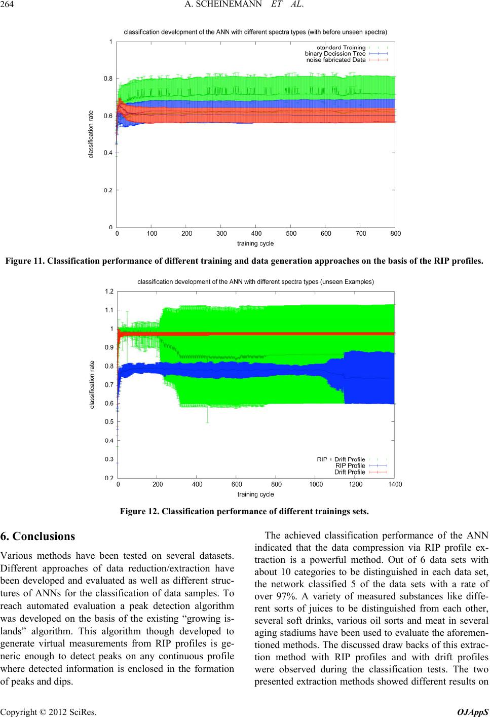

A. SCHEINEMANN ET AL. 264
Figure 11. Classification performance of different training and data generation approaches on the basis of the RIP profiles.
Figure 12. Classification performance of different trainings sets.
ave been tested on several datasets.
n performance of the ANN
o be distinguished in each data set,
th
6. Conclusions
Various methods h
Different approaches of data reduction/extraction have
been developed and evaluated as well as different struc-
tures of ANNs for the classification of data samples. To
reach automated evaluation a peak detection algorithm
was developed on the basis of the existing “growing is-
lands” algorithm. This algorithm though developed to
generate virtual measurements from RIP profiles is ge-
neric enough to detect peaks on any continuous profile
where detected information is enclosed in the formation
of peaks and dips.
indicated that the data compression via RIP profile ex-
traction is a powerful method. Out of 6 data sets with
about 10 categories t
The achieved classificatio
e network classified 5 of the data sets with a rate of
over 97%. A variety of measured substances like diffe-
rent sorts of juices to be distinguished from each other,
several soft drinks, various oil sorts and meat in several
aging stadiums have been used to evaluate the aforemen-
tioned methods. The discussed draw backs of this extrac-
tion method with RIP profiles and with drift profiles
were observed during the classification tests. The two
presented extraction methods showed different results on

A. SCHEINEMANN ET AL. 265
the available data sets. In the end at least one strategy for
every available classification problem was found, which
managed to reach high classification rates. The combined
classification results of RIP profiles and drift profiles are
encouraging. Since they lay ground for automated eva-
luation of measurements and possible monitoring appli-
cations.
An overview of the reached classification results with
the different evaluation strategies is given in Table 2. The
classification rates given in this table are maximum rates
that were reached during several training attempts.
en-
tio
r data extraction and d
re
re relevant data
se
Classification rate
One disadvantage was already mentioned in the intro-
duction. Though the RIP profile contains information
about peaks being measured in the GC-IMS spectrum it
doesn’t show double peaks appearing at the same ret
n time, which arise from monomer and dimer forma-
tion. Another drawback is the loss of information on the
drift time of the peaks. This can lead to the creation of
RIP profiles without any discriminating information.
This is the reason why in some cases the drift profiles
achieve better classification results. Since the principle is
the same, information appears in form of the peaks, the
profiles are interchangeable.
Further Improvements: Although this paper shows
great potential in evaluation of GC-IMS measurements
with ANNs, there are still improvements possible which
are to be investigated. Otheata
duction methods should be considered.
Furthermore tests with bigger data sets should be im-
plemented to investigate the convergence and the classi-
fication behavior of the ANNs and the according data
extraction strategies. Only statistically mo
ts are able to determine the stableness and usability of
this method.
Table 2. Classification rates for all measured data with dif-
ferent training profiles used to train the ANN.
Measurement Drift profiles RIP profiles
Cola 91.0% 96.3%
Juice 88.8%
oil
flavors
meat
98.6%
Rice 100% 100%
Olive 98.9% 76.4%
Candy100% 100%
Aging96.6% 100%
7. Acknowledgements
his work has been supported by the German BMBF,
contract 01IS09046A.
Mobility Spectrometry,” Taylor and
Francis Group, London, 2005.
doi:10.1201/97
T
REFERENCES
[1] G. A. Eiceman, “Ion
81420038972
[2] M. Tsvet, “Physical Chemical Studies on Chlorophyll
Adsorptions,” Berichte der Deutschen Botanischen Ge-
sellschaft, Vol. 24, 1906, pp. 316-323.
etry, Vol. 402, No. 1, 2012, pp. 489-498.
l for Ion Mobility Spectrometry, Vol. 4,
[3] F. W. Cohen and M. J. Karasek, “Plasma Chromatogra-
phy—A New Dimension for Gas Chromatography and
Mass Spectrometry,” Journal of Chromatographic Sci-
ence, Vol. 8, No. 6, 1970, pp. 330-337.
[4] C. P. Cram and S. N. Chesler, “Coupling of High Speed
Plasma Chromatography with Gas Chromatography,” Jour-
nal of Chromatographic Science, Vol. 11, No. 8, 1973, pp.
391-401.
[5] B. Bodeker and J. I. Baumbach, “Analytical Description
of IMS-Signals,” International Journal for Ion Mobility
Spectrometry, Vol. 12, No. 3, 2009, pp. 103-108.
[6] J. Xu and B. W. William, “Monte Carlo Simulation of Ion
Transport in Ion Mobility Spectrometry,” International
Journal for Ion Mobility Spectrometry, Vol. 11, No. 1-4,
2008, pp. 13-17.
[7] J. I. Baumbach, S. Sielemann and P. Pilzecker, “Coupling
of Multi-Capillary Columns with Two Dierent Types of
Ion Mobility Spectrometer,” International Journal for Ion
Mobility Spectrom
[8] C. L. P. Thomas, “Sensitivity and Resolution in Gas Chro-
matography-Ion Mobility Spectrometry,” International
Journal for Ion Mobility Spectrometry, Vol. 4, No. 2,
2001, pp. 62-68.
[9] Z. Xie, S. Sielemann, H. Schmidt and J. I. Baumbach, “A
Novel Method for the Detection of MTBE: Ion Mobility
Spectrometry Coupled to Multi Capillary Column,” In-
ternational Journa
No. 1, 2000, pp. 77-86.
[10] R. Rojas, “Neural Networks,” Springer, Berlin, Heidel-
berg, 1996.
[11] R. L. Harvey, “Neural Network Principles,” Prentice-Hall
International, Upper Saddle River, 1994.
[12] F. Gerald, “Curves and Surfaces for Computer-Aided
Geometric Design,” 4th Edition, Elsevier Science and
Technology Books, Amsterdam, 1997.
[13] D. Lasser, “Bernstein-Bezier Representation of Volumes,”
Computer Aided Geometric Design, Vol. 2, No. 1-3, 1985,
pp. 145-149.

A. SCHEINEMANN ET AL. 266
Nomenclature
Description Symbol
R
t Retention time
D
t Drift time
,max ,max
,
RD
tt Measurement specific maximal values of retention or drift time

,
RD
I
tt ,

,
iRD
R
tt ,

,
RD

M
tt
2-dimensio
representat
nal matrix representation of a MCC-IMS measurement, in some cases this discrete data
ion is regarded as continuous, which is justified by the high resolution due to a high
sampling rate in the available measurements

R
Qt Complete charge accumulated at one certain retention time by summing up charge at all drift times



,, ,
iRDjRD
R
tt Rtt Function mapping 2 matrices i
R
and j
R
of identical dimension to a scalar value

:, ,
iRDjRD
Rtt Rtt

D
D
t 1-dimensional extraction of a pfile alo the drift time axis ro ng

iR
F
t Partition of a 1-dimensional proffiles that contain only one extre
file
ile into peace wise promum which is not located
on the edge points of this pro

n
B
t Bezier curve of order n defined by n + 1 control points