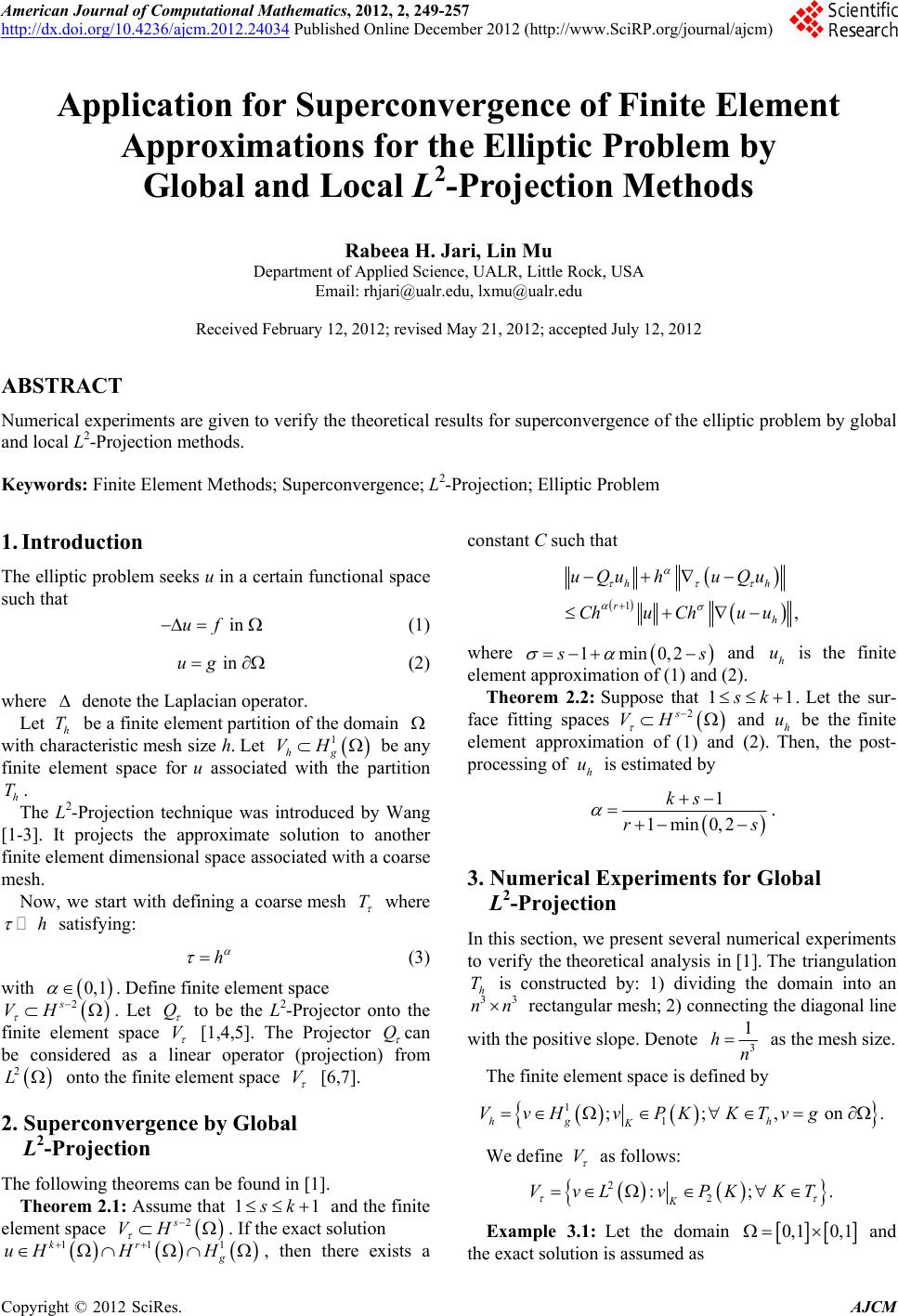
American Journal of Computational Mathematics, 2012, 2, 249-257
http://dx.doi.org/10.4236/ajcm.2012.24034 Published Online December 2012 (http://www.SciRP.org/journal/ajcm)
Application for Superconvergence of Finite Element
Approximations for the Elliptic Problem by
Global and Local L2-Projection Methods
Rabeea H. Jari, Lin Mu
Department of Applied Science, UALR, Little Rock, USA
Received February 12, 2012; revised May 21, 2012; accepted July 12, 2012
ABSTRACT
Numerical experiments are given to verify the theoretical results for superconvergence of the elliptic problem by global
and local L2-Projection methods.
Keywords: Finite Element Methods; Superconvergence; L2-Projection; Elliptic Problem
1. Introduction
The elliptic problem seeks u in a certain functional space
such that
in uf (1)
in ug (2)
where denote the Laplacian operator.

Let h be a finite element partition of the domain T

with characteristic mesh size h. Let be any
finite element space for u associated with the partition
.

1
hg
VH
h
T
The L2-Projection technique was introduced by Wang
[1-3]. It projects the approximate solution to another
finite element dimensional space associated with a coarse
mesh.
Now, we start with defining a coarse mesh T

where
h

 satisfying:
h

  (3)
with . Define finite element space

. Let

0,1  

2s
VH



Q

to be the L2-Projector onto the
finite element space V

[1,4,5]. The Projector Q

can
be considered as a linear operator (projection) from
onto the finite element space

2
L

V

[6,7].
2. Superconvergence by Global
L2-Projection
The following theorems can be found in [1].
Theorem 2.1: Assume that 11
s
k


and the finite
element space . If the exact solution

2s
VH






1

11krg
H H

uH , then there exists a
constant C such that



1,
hh
rh
uQu huQu
ChuChu u






where


1min0,2
s
s 

 and is the finite
element approximation of (1) and (2).
h
u
Theorem 2.2: Suppose that 11
s
k

u. Let the sur- face fitting spaces and h be the finite
element approximation of (1) and (2). Then, the post-
processing of is estimated by
2s
VH



h
u

1
1min0,2
ks
rs





.
3. Numerical Experiments for Global
L2-Projection
In this section, we present several numerical experiments
to verify the theoretical analysis in [1]. The triangulation
is constructed by: 1) dividing the domain into an
h
T
n
3
n
3

rectangular mesh; 2) connecting the diagonal line
with the positive slope. Denote 3
1
hn  as the mesh size.
The finite element space is defined by






1
1
;; , on
hg h
K
VvH vPKKTvg.

 
We define V

as follows:




2
2
:;
K
VvLvPKKT

  .
Example 3.1: Let the domain




0,1 0,1  and
the exact solution is assumed as
C
opyright © 2012 SciRes. AJCM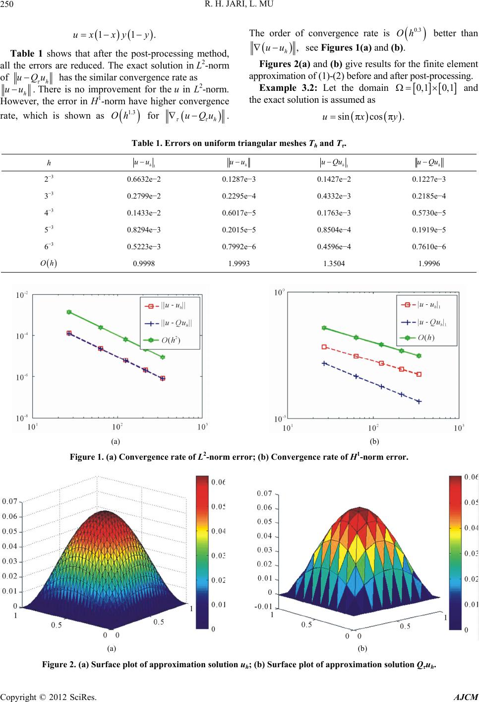

R. H. JARI, L. MU 250

11ux xyy .
Table 1 shows that after the post-processing method,
all the errors are reduced. The exact solution in L2-norm
of h uQu

 has the similar convergence rate as
h
uu. There is no improvement for the u in L2-norm.
However, the error in H1-norm have higher convergence
rate, which is shown as


1.3
Oh for

h
uQu

 .
The order of convergence rate is better than

0.3
Oh



,
h
uu see Figures 1(a) and (b).
Figures 2(a) and (b) give results for the finite element
approximation of (1)-(2) before and after post-processing.
Example 3.2: Let the domain




0,1 0,1  and
the exact solution is assumed as


sin πcos π.uxy
Table 1. Errors on uniform triangular meshes Th and Tτ.
h 1
h
uu h uu 1
h
uQu h uQu
2−3 0.6632e−2 0.1287e−3 0.1427e−2 0.1227e−3
3−3 0.2799e−2 0.2295e−4 0.4332e−3 0.2185e−4
4−3 0.1433e−2 0.6017e−5 0.1763e−3 0.5730e−5
5−3 0.8294e−3 0.2015e−5 0.8504e−4 0.1919e−5
6−3 0.5223e−3 0.7992e−6 0.4596e−4 0.7610e−6

Oh 0.9998 1.9993 1.3504 1.9996
(a) (b)
Figure 1. (a) Convergence rate of L2-norm error; (b) Convergence rate of H1-norm error.
(a) (b)
Figure 2. (a) Surface plot of approximation solution uh; (b) Surface plot of approximation solution Qτuh.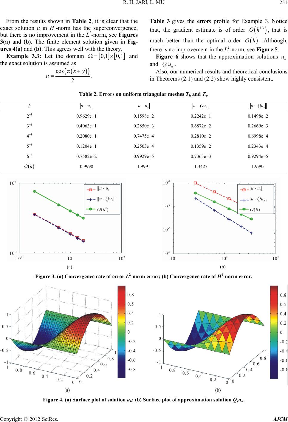

R. H. JARI, L. MU 251
From the results shown in Table 2, it is clear that the
exact solution u in H1-norm has the superconvergence,
but there is no improvement in the L2-norm, see Figures
3(a) and (b). The finite element solution given in Fig-
ures 4(a) and (b). This agrees well with the theory.
Example 3.3: Let the domain




0,1 0,1  and
the exact solution is assumed as



cos π
.
2
x
y
u 
Table 3 gives the errors profile for Example 3. Notice
that, the gradient estimate is of order , that is

1.3
Oh

much better than the optimal order . Although,
there is no improvement in the L2-norm, see Figure 5.

Oh
Figure 6 shows that the approximation solutions
and .
h
u
h 
Also, our numerical results and theoretical conclusions
in Theorems (2.1) and (2.2) show highly consistent.
Qu
Table 2. Errors on uniform triangular meshes Th and Tτ.
h 1
h
uu h uu 1
h
uQu h uQu
2−3 0.9629e−1 0.1598e−2 0.2242e−1 0.1498e−2
3−3 0.4063e−1 0.2850e−3 0.6872e−2 0.2669e−3
4−3 0.2080e−1 0.7475e−4 0.2810e−2 0.6998e−4
5−3 0.1204e−1 0.2503e−4 0.1359e−2 0.2343e−4
6−3 0.7582e−2 0.9929e−5 0.7363e−3 0.9294e−5

Oh 0.9998 1.9991 1.3427 1.9995
(a) (b)
Figure 3. (a) Convergence rate of error L2-norm error; (b) Convergence rate of H1-norm error.
(a) (b)
Figure 4. (a) Surface plot of solution uh; (b) Surface plot of approximation solution Qτuh.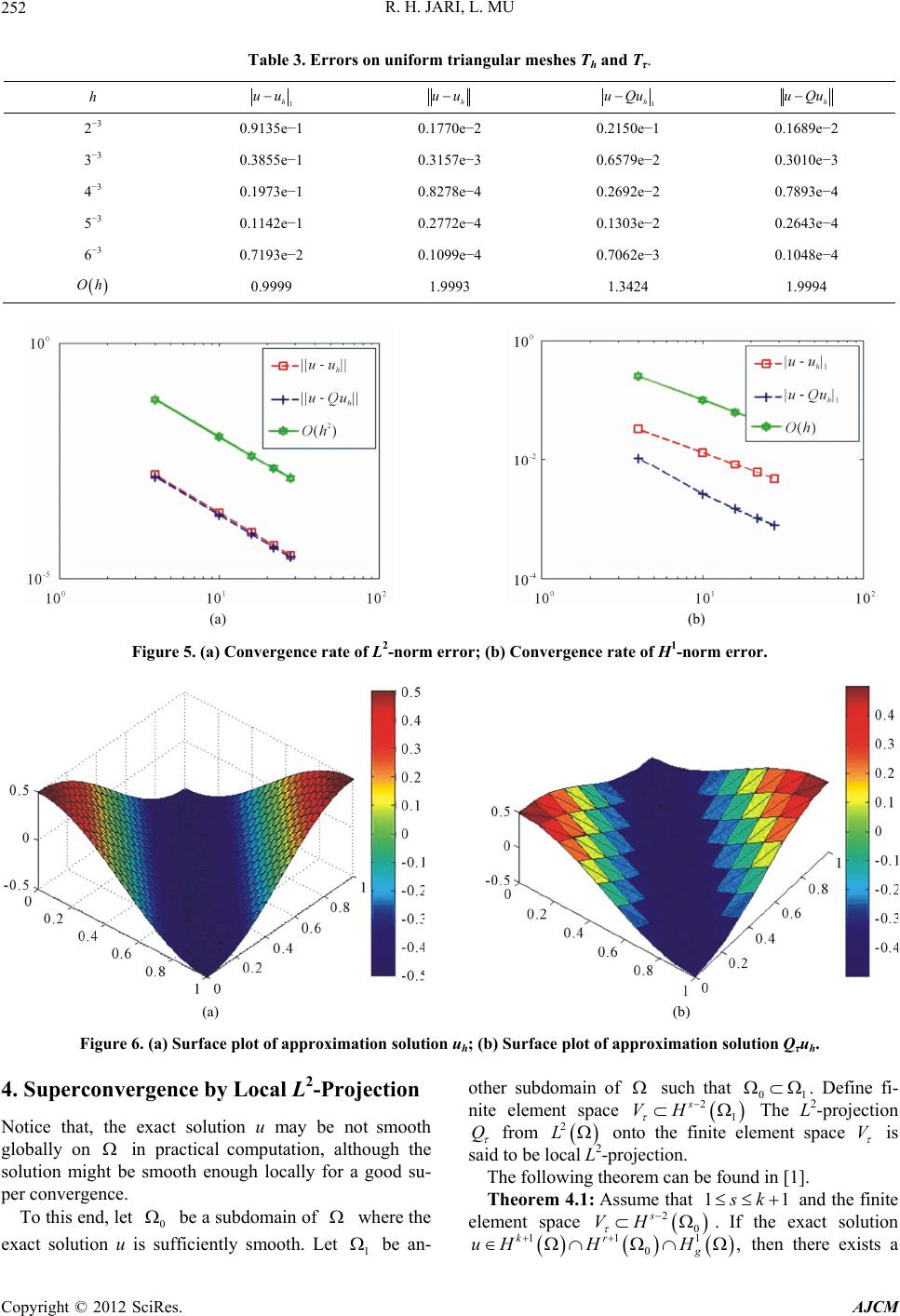

R. H. JARI, L. MU 252
Table 3. Errors on uniform triangular meshes Th and Tτ.
h 1
h
uu h uu 1
h
uQu h uQu
2−3 0.9135e−1 0.1770e−2 0.2150e−1 0.1689e−2
3−3 0.3855e−1 0.3157e−3 0.6579e−2 0.3010e−3
4−3 0.1973e−1 0.8278e−4 0.2692e−2 0.7893e−4
5−3 0.1142e−1 0.2772e−4 0.1303e−2 0.2643e−4
6−3 0.7193e−2 0.1099e−4 0.7062e−3 0.1048e−4

Oh 0.9999 1.9993 1.3424 1.9994
(a) (b)
Figure 5. (a) Convergence rate of L2-norm error; (b) Convergence rate of H1-norm error.
(a) (b)
Figure 6. (a) Surface plot of approximation solution uh; (b) Surface plot of approximation solution Qτuh.
4. Superconvergence by Local L2-Projection
Notice that, the exact solution u may be not smooth
globally on in practical computation, although the
solution might be smooth enough locally for a good su-
per convergence.

To this end, let be a subdomain of where the
0

exact solution u is sufficiently smooth. Let be an-
1

other subdomain of

such that 01 . Define fi-
nite element space The L2-projection




2
1
s
VH



Q

from


2
L

onto the finite element space V

is
said to be local L2-projection.
The following theorem can be found in [1].
Theorem 4.1: Assume that 11
s
k and the finite
element space



2
0
s
VH


. If the exact solution




11
0
kr
H H


1
,
g
uH

 then there exists a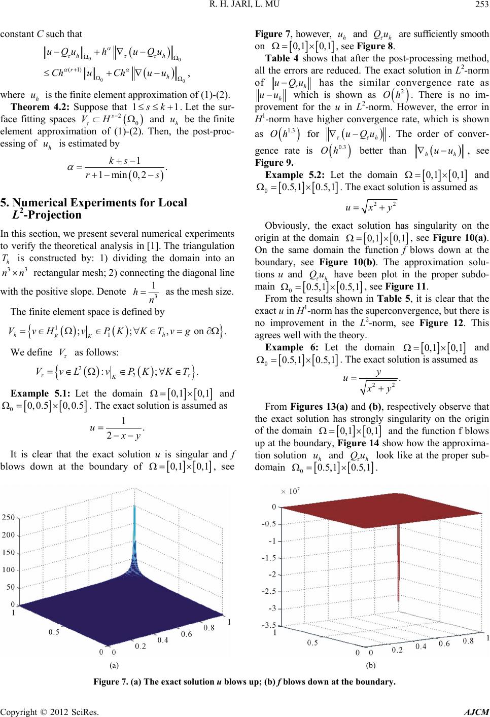

R. H. JARI, L. MU 253
constant C such that



00
00
(1) ,
hh
rh
uQu huQu
ChuChu u








where is the finite element approximation of (1)-(2).
h
Theorem 4.2: Suppose that 1
u
1
s
k. Let the sur-
face fitting spaces


0
u
2s
VH


 and h be the finite
element approximation of (1)-(2). Then, the post-proc-
essing of is estimated by
h
u

1.
1min0,2
ks
rs



5. Numerical Experiments for Local
L2-Projection
In this section, we present several numerical experiments
to verify the theoretical analysis in [1]. The triangulation
is constructed by: 1) dividing the domain into an
h
T
3
nn3 rectangular mesh; 2) connecting the diagonal line
with the positive slope. Denote 3
1
hn  as the mesh size.
The finite element space is defined by
 

1
1
;;, on .
hg h
K
VvH vPKKTvg 

We define V

as follows:
 

2
2
:;
K
VvL vPKKT

.
Example 5.1: Let the domain




0,1 0,1  and




00, 0.50, 0.5 . The exact solution is assumed as
1.
2
u
x
y

It is clear that the exact solution u is singular and f
blows down at the boundary of




0,1 0,1  , see
Figure 7, however, h and h Qu

are sufficiently smooth
on
u




0,1 0,1 , see Figure 8.
Table 4 shows that after the post-processing method,
all the errors are reduced. The exact solution in L2-norm
of h
uQu

 has the similar convergence rate as
h
uu which is shown as . There is no im-
provement for the u in L2-norm. However, the error in
H1-norm have higher convergence rate, which is shown

2
Oh
as


1.3
Oh for


h
uQu

 . The order of conver-
gence rate is


0.3
Oh better than

hh
uu, see
Figure 9.




Example 5.2: Let the domain 0,1 0,1  and




00.5,1 0.5,1  . The exact solution is assumed as
22
uxy
Obviously, the exact solution has singularity on the
origin at the domain




0,1 0,1  , see Figure 10(a).
On the same domain the function f blows down at the
boundary, see Figure 10(b). The approximation solu-
tions u and have been plot in the proper subdo-
main
h
Qu





0
From the results shown in Table 5, it is clear that the
exact u in H1-norm has the superconvergence, but there is
no improvement in the L2-norm, see Figure 12. This
agrees well with the theory.
0.5,1 0.5,1  , see Figure 11.
Example 6: Let the domain




0,1 0,1  and




00.5,1 0.5,1  . The exact solution is assumed as
22
.
y
u
x
y


From Figures 13(a) and (b), respectively observe that
the exact solution has strongly singularity on the origin
of the domain




0,1 0,1 
h
uh Qu

and the function f blows
up at the boundary, Figure 14 show how the approxima-
tion solution and look like at the proper sub-
domain




0
0.5,1 0.5,1.
(a) (b)
Figure 7. (a) The exact solution u blows up; (b) f blows down at the boundary.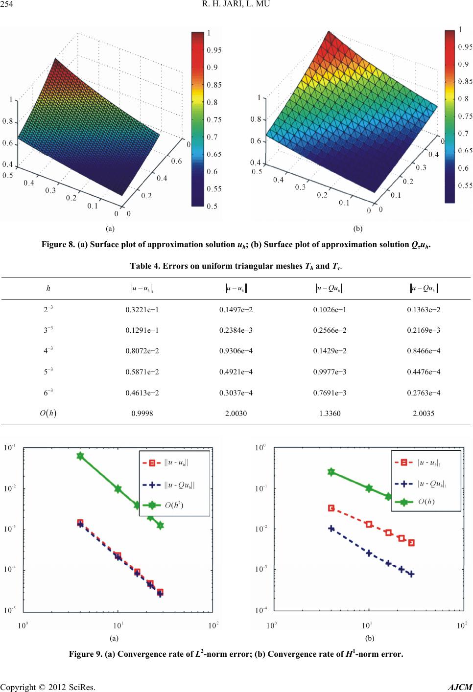

R. H. JARI, L. MU 254
(a) (b)
Figure 8. (a) Surface plot of approximation solution uh; (b) Surface plot of approximation solution Qτuh.
Table 4. Errors on uniform triangular meshes Th and Tτ.
h 1
h
uu h uu 1
h
uQu h uQu
2−3 0.3221e−1 0.1497e−2 0.1026e−1 0.1363e−2
3−3 0.1291e−1 0.2384e−3 0.2566e−2 0.2169e−3
4−3 0.8072e−2 0.9306e−4 0.1429e−2 0.8466e−4
5−3 0.5871e−2 0.4921e−4 0.9977e−3 0.4476e−4
6−3 0.4613e−2 0.3037e−4 0.7691e−3 0.2763e−4

Oh 0.9998 2.0030 1.3360 2.0035
(a) (b)
Figure 9. (a) Convergence rate of L2-norm error; (b) Convergence rate of H1-norm error.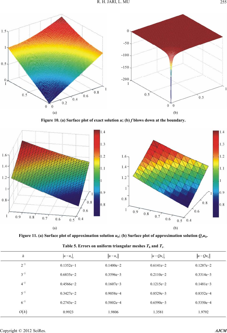

R. H. JARI, L. MU 255
(a) (b)
Figure 10. (a) Surface plot of exact solution u; (b) f blows down at the boundary.
(a) (b)
Figure 11. (a) Surface plot of approximation solution uh; (b) Surface plot of approximation solution Qτuh.
Table 5. Errors on uniform triangular meshes Th and Tτ.
h 1
h
uu h uu 1
h
uQu h uQu
2−3 0.1352e−1 0.1400e−2 0.6141e−2 0.1287e−2
3−3 0.6835e−2 0.3596e−3 0.2110e−2 0.3314e−3
4−3 0.4566e−2 0.1607e−3 0.1215e−2 0.1481e−3
5−3 0.3427e−2 0.9058e−4 0.8529e−3 0.8352e−4
6−3 0.2743e−2 0.5802e−4 0.6590e−3 0.5350e−4

Oh 0.9923 1.9806 1.3581 1.9792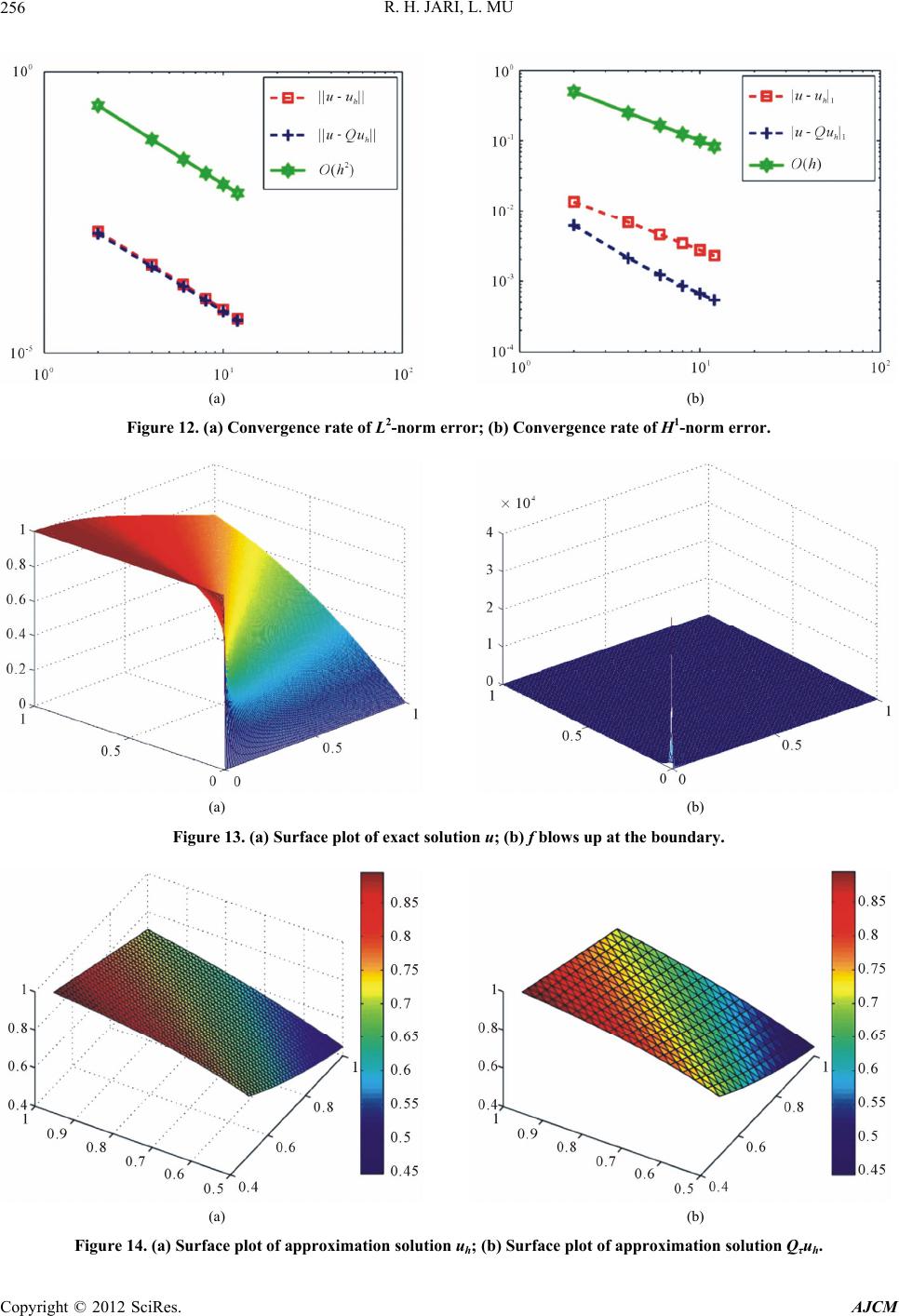

R. H. JARI, L. MU 256
(a) (b)
Figure 12. (a) Convergence rate of L2-norm error; (b) Convergence rate of H1-norm error.
(a) (b)
Figure 13. (a) Surface plot of exact solution u; (b) f blows up at the boundary .
(a) (b)
Figure 14. (a) Surface plot of approximation solution uh; (b) Surface plot of approximation solution Qτuh.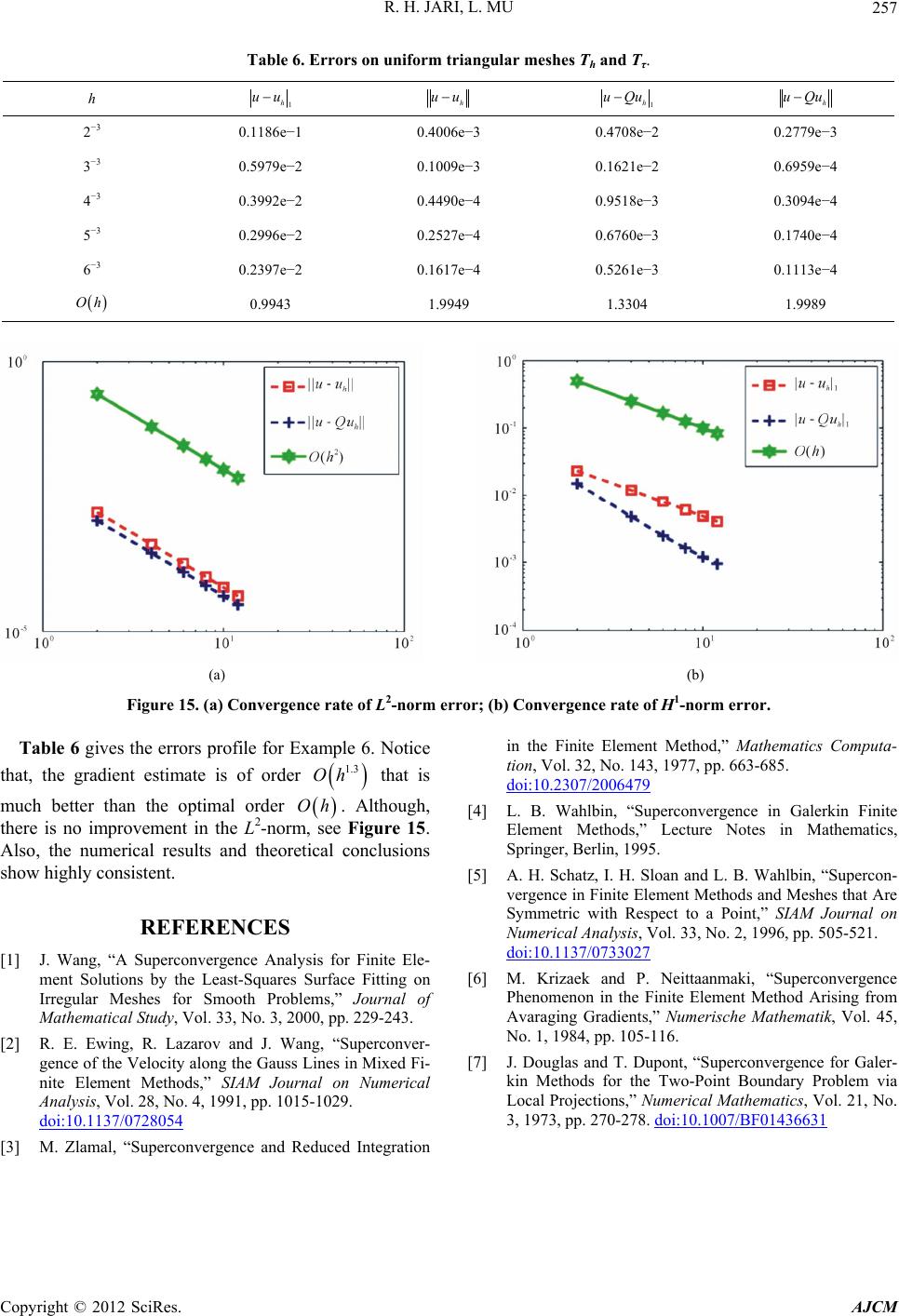

R. H. JARI, L. MU 257
Table 6. Errors on uniform triangular meshes Th and Tτ.
h 1
h
uu h uu 1
h
uQu h uQu
2−3 0.1186e−1 0.4006e−3 0.4708e−2 0.2779e−3
3−3 0.5979e−2 0.1009e−3 0.1621e−2 0.6959e−4
4−3 0.3992e−2 0.4490e−4 0.9518e−3 0.3094e−4
5−3 0.2996e−2 0.2527e−4 0.6760e−3 0.1740e−4
6−3 0.2397e−2 0.1617e−4 0.5261e−3 0.1113e−4

Oh 0.9943 1.9949 1.3304 1.9989
(a) (b)
Figure 15. (a) Convergence rate of L2-norm error; (b) Convergence rate of H1-norm error.
Table 6 gives the errors profile for Example 6. Notice
that, the gradient estimate is of order that is

1.3
Oh

much better than the optimal order . Although,
there is no improvement in the L2-norm, see Figure 15.
Also, the numerical results and theoretical conclusions
show highly consistent.

Oh
REFERENCES
[1] J. Wang, “A Superconvergence Analysis for Finite Ele-
ment Solutions by the Least-Squares Surface Fitting on
Irregular Meshes for Smooth Problems,” Journal of
Mathematical Study, Vol. 33, No. 3, 2000, pp. 229-243.
[2] R. E. Ewing, R. Lazarov and J. Wang, “Superconver-
gence of the Velocity along the Gauss Lines in Mixed Fi-
nite Element Methods,” SIAM Journal on Numerical
Analysis, Vol. 28, No. 4, 1991, pp. 1015-1029.
doi:10.1137/0728054
[3] M. Zlamal, “Superconvergence and Reduced Integration
in the Finite Element Method,” Mathematics Computa-
tion, Vol. 32, No. 143, 1977, pp. 663-685.
doi:10.2307/2006479
[4] L. B. Wahlbin, “Superconvergence in Galerkin Finite
Element Methods,” Lecture Notes in Mathematics,
Springer, Berlin, 1995.
[5] A. H. Schatz, I. H. Sloan and L. B. Wahlbin, “Supercon-
vergence in Finite Element Methods and Meshes that Are
Symmetric with Respect to a Point,” SIAM Journal on
Numerical Analysis, Vol. 33, No. 2, 1996, pp. 505-521.
doi:10.1137/0733027
[6] M. Krizaek and P. Neittaanmaki, “Superconvergence
Phenomenon in the Finite Element Method Arising from
Avaraging Gradients,” Numerische Mathematik, Vol. 45,
No. 1, 1984, pp. 105-116.
[7] J. Douglas and T. Dupont, “Superconvergence for Galer-
kin Methods for the Two-Point Boundary Problem via
Local Projections,” Numerical Mathematics, Vol. 21, No.
3, 1973, pp. 270-278. doi:10.1007/BF01436631