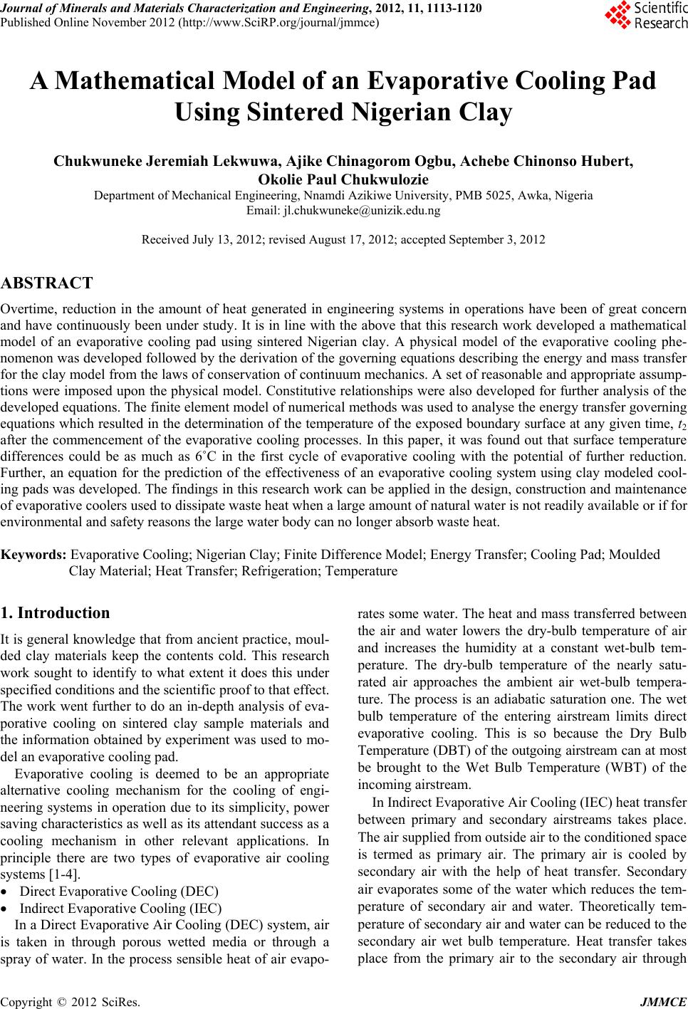Journal of Minerals and Materials Characterization and Engineering, 2012, 11, 1113-1120
Published Online November 2012 (http://www.SciRP.org/journal/jmmce)
A Mathematical Model of an Evaporative Cooling Pad
Using Sintered Nigerian Clay
Chukwuneke Jeremiah Lekwuwa, Ajike Chinagorom Ogbu, Achebe Chinonso Hubert,
Okolie Paul Chukwulozie
Department of Mechanical Engineering, Nnamdi Azikiwe University, PMB 5025, Awka, Nigeria
Received July 13, 2012; revised August 17, 2012; accepted September 3, 2012
ABSTRACT
Overtime, reduction in the amount of heat generated in engineering systems in operations have been of great concern
and have continuously been under study. It is in line with the above that this research work developed a mathematical
model of an evaporative cooling pad using sintered Nigerian clay. A physical model of the evaporative cooling phe-
nomenon was developed followed by the derivation of the governing equations describing the energy and mass transfer
for the clay model from the laws of conservation of continuum mechanics. A set of reasonable and appropriate assump-
tions were imposed upon the physical model. Constitutive relationships were also developed for further analysis of the
developed equations. The finite element model of numerical methods was used to analyse the energy transfer governing
equations which resulted in the determination of the temperature of the exposed boundary surface at any given time, t2
after the commencement of the evaporative cooling processes. In this paper, it was found out that surface temperature
differences could be as much as 6˚C in the first cycle of evaporative cooling with the potential of further reduction.
Further, an equation for the prediction of the effectiveness of an evaporative cooling system using clay modeled cool-
ing pads was developed. The findings in this research work can be applied in the design, construction and maintenance
of evaporative coolers used to dissipate waste heat when a large amount of natural water is not readily available or if for
environmental and safety reasons the large water body can no longer absorb waste heat.
Keywords: Evaporative Cooling; Nigerian Clay; Finite Difference Model; Energy Transfer; Cooling Pad; Moulded
Clay Material; Heat Transfer; Refrigeration; Temperature
1. Introduction
It is general knowledge that from ancient practice, moul-
ded clay materials keep the contents cold. This research
work sought to identify to what extent it does this under
specified conditions and the scientific proof to that effect.
The work went further to do an in-depth analysis of eva-
porative cooling on sintered clay sample materials and
the information obtained by experiment was used to mo-
del an evaporative cooling pad.
Evaporative cooling is deemed to be an appropriate
alternative cooling mechanism for the cooling of engi-
neering systems in operation due to its simplicity, power
saving characteristics as well as its attendant success as a
cooling mechanism in other relevant applications. In
principle there are two types of evaporative air cooling
systems [1-4].
 Direct Evaporative Cooling (DEC)
 Indirect Evaporative Cooling (IEC)
In a Direct Evaporative Air Cooling (DEC) system, air
is taken in through porous wetted media or through a
spray of water. In the process sensible heat of air evapo-
rates some water. The heat and mass transferred between
the air and water lowers the dry-bulb temperature of air
and increases the humidity at a constant wet-bulb tem-
perature. The dry-bulb temperature of the nearly satu-
rated air approaches the ambient air wet-bulb tempera-
ture. The process is an adiabatic saturation one. The wet
bulb temperature of the entering airstream limits direct
evaporative cooling. This is so because the Dry Bulb
Temperature (DBT) of the outgoing airstream can at most
be brought to the Wet Bulb Temperature (WBT) of the
incoming airstream.
In Indirect Evaporative Air Cooling (IEC) heat transfer
between primary and secondary airstreams takes place.
The air supplied from outside air to the conditioned space
is termed as primary air. The primary air is cooled by
secondary air with the help of heat transfer. Secondary
air evaporates some of the water which reduces the tem-
perature of secondary air and water. Theoretically tem-
perature of secondary air and water can be reduced to the
secondary air wet bulb temperature. Heat transfer takes
place from the primary air to the secondary air through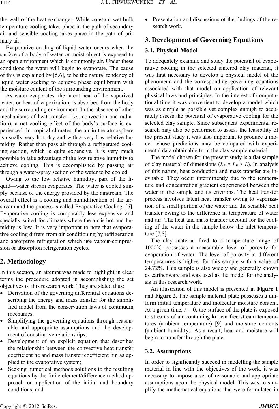

J. L. CHWUKWUNEKE ET AL.
1114
the wall of the heat exchanger. While constant wet bulb
temperature cooling takes place in the path of secondary
air and sensible cooling takes place in the path of pri-
mary air.
Evaporative cooling of liquid water occurs when the
surface of a body of water or moist object is exposed to
an open environment which is commonly air. Under these
conditions the water will begin to evaporate. The cause
of this is explained by [5,6], to be the natural tendency of
liquid water seeking to achieve phase equilibrium with
the moisture content of the surrounding environment.
As water evaporates, the latent heat of the vaporized
water, or heat of vaporization, is absorbed from the body
and the surrounding environment. In the absence of other
mechanisms of heat transfer (i.e., convection and radia-
tion), a net cooling effect of the body’s surface is ex-
perienced. In tropical climates, the air in the atmosphere
is usually very hot, dry and with a very low relative hu-
midity. Rather than pass air through a refrigerated cool-
ing section, which is quite expensive, it is very much
possible to take advantage of the low relative humidity to
achieve cooling. This is accomplished by passing air
through a water-spray section of the water to be cooled.
Owing to the low relative humidity, part of the li-
quid—water stream evaporates. The water is cooled sim-
ply because of the energy provided by the airstream. The
overall effect is a cooling and humidification of the air-
stream and the process is called Evaporative Cooling, [6].
Evaporative cooling is comparably less expensive and
specially suited for climates where the air is hot and hu-
midity is low. It is very important to note that evapora-
tive cooling differs from air conditioning by refrigeration
and absorptive refrigeration which use vapour-compres-
sion or absorption refrigeration cycles.
2. Methodology
In this section, an attempt was made to highlight in clear
terms the procedure adopted in accomplishing the set
objectives of this research work. They are stated thus:
 Derivation of the governing differential equations de-
scribing the energy and mass transfer for the simpli-
fied model from the conservation laws of continuum
mechanics;
 Simplifying the governing equations through reason-
able and appropriate assumptions and the develop-
ment of constitutive relationships;
 Development of an explicit equation that describes
the relationship between the convective heat transfer
coefficient hc and mass transfer coefficient hm as ap-
plied to the evaporative system;
 Seeking numerical methods solutions to the resulting
equations by the finite element/difference method ap-
proach on application of the initial and boundary
conditions; and
 Presentation and discussions of the findings of the re-
search work.
3. Development of Governing Equations
3.1. Physical Model
To adequately examine and study the potential of evapo-
rative cooling in the selected sintered clay material, it
was first necessary to develop a physical model of the
phenomena and the corresponding governing equations
associated with that model on application of relevant
physical laws and principles. In the interest of computa-
tional time it was convenient to develop a model which
was as simple as possible yet complex enough to accu-
rately assess the potential of evaporative cooling for the
selected clay sample. Since subsequent experimental re-
search may also be performed to assess the feasibility of
the present study it was also important to produce a mo-
del whose predictions may be compared with experi-
mental data obtainable from the clay sample material.
The model chosen for the present study is a flat sample
of clay material of dimensions (LP × LP × L). In analysis
of this nature, heat conduction and mass transfer are in-
evitable. They occur intermittently due to the tempera-
ture and concentration gradient experienced between the
water in the sample and its environs. The heat transfer
process involves latent heat transfer owing to vaporiza-
tion of a small portion of the water and the sensible heat
transfer owing to the difference in temperature of water
and air. The heat and mass transfer account for the cool-
ing of the water in the sample below the inlet tempera-
ture [7,8].
The clay material fired to a temperature range of
1000˚C possesses a measurable level of porosity for
evaporation of water. The level of porosity at different
temperatures is highest for this sample with a value of
24.72%. This sample is also widely and generally known
as earthenware and was used as the model for the analy-
sis in this research work.
An illustration of this model is presented in Figure 1
and Figure 2. The sample material plate possesses a uni-
form initial temperature and molecular moisture content.
At a given time, t = 0, the surface of the plate is exposed
to streams of air containing known free stream tempera-
tures (ambient temperature) [9] and moisture contents
(ambient humidity). As a result, heat and moisture will
begin to transfer through the plate.
3.2. Assumptions
In order to significantly succeed in modelling the sample
material in line with the objectives of the work, it was
necessary to impose a set of reasonable and appropriate
assumptions upon the physical model. This was to sim-
plify the mathematical equations that were formulated in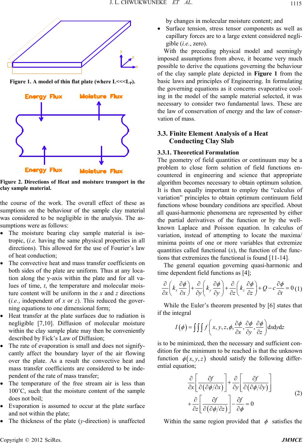

J. L. CHWUKWUNEKE ET AL. 1115
y
z
x
Figure 1. A model of thi n fl at plate (where L<<<L P).

Figure 2. Directions of Heat and moisture transport in the
clay sample material.
the course of the work. The overall effect of these as
sumptions on the behaviour of the sample clay material
was considered to be negligible in the analysis. The as-
sumptions were as follows:
 The moisture bearing clay sample material is iso-
tropic, (i.e. having the same physical properties in all
directions). This allowed for the use of Fourier’s law
of heat conduction;
 The convective heat and mass transfer coefficients on
both sides of the plate are uniform. Thus at any loca-
tion along the y-axis within the plate and for all va-
lues of time, t, the temperature and molecular mois-
ture content will be uniform in the x and z directions
(i.e., independent of x or z). This reduced the gover-
ning equations to one dimensional form;
 Heat transfer at the plate surfaces due to radiation is
negligible [7,10]. Diffusion of molecular moisture
within the clay sample plate may then be conveniently
described by Fick’s Law of Diffusion;
 The rate of evaporation is small and does not signify-
cantly affect the boundary layer of the air flowing
over the plate. As a result the convective heat and
mass transfer coefficients are considered to be inde-
pendent of the rate of mass transfer;
 The temperature of the free stream air is less than
100˚C, such that the moisture content of the sample
does not boil;
 Evaporation is assumed to occur at the plate surface
and not within the plate;
 The thickness of the plate (y-direction) is unaffected
by changes in molecular moisture content; and
 Surface tension, stress tensor components as well as
capillary forces are to a large extent considered negli-
gible (i.e., zero).
With the preceding physical model and seemingly
imposed assumptions from above, it became very much
possible to derive the equations governing the behaviour
of the clay sample plate depicted in Figure 1 from the
basic laws and principles of Engineering. In formulating
the governing equations as it concerns evaporative cool-
ing in the model of the sample material selected, it was
necessary to consider two fundamental laws. These are
the law of conservation of energy and the law of conser-
vation of mass.
3.3. Finite Element Analysis of a Heat
Conducting Clay Slab
3.3.1. Theoretical Formulation
The geometry of field quantities or continuum may be a
problem to close form solution of field functions en-
countered in engineering and science that appropriate
algorithm becomes necessary to obtain optimum solution.
It is then equally important to employ the “calculus of
variation” principles to obtain optimum continuum field
functions whose boundary conditions are specified. About
all quasi-harmonic phenomena are represented by either
the partial derivatives of the function or by the well-
known Laplace and Poisson equation. In calculus of
variation, instead of attempting to locate the maxima/
minima points of one or more variables that extremize
quantities called functional (x), the function of the func-
tions that extremizes the functional is found [11-14].
The general equation governing quasi-harmonic and
time dependent field functions as [4];
0
xyz
kkkQc
xxyyzz t
    
 




 
 
 
 
(1)
While the Euler’s theorem presented by [6] states that
if the integral

,,,,,,ddd
I
f xyzxyz
xyz








is to be minimized, then the necessary and sufficient con-
dition for the minimum to be reached is that the unknown
function


,,
x
yz 
should satisfy the following differ-
ential equation;
 

0
ff
x
xy y
ff
zz




 



  

 



 


 



(2)
Within the same region provided that

satisfies the

J. L. CHWUKWUNEKE ET AL.
1116
same boundary condition in both cases. From the on-
going, it can be shown that the equivalent formulation to
that of Equation (1) is the requirement that the volume
integral given below and taken over the whole region,
should be minimized.
2
22
1
2xyz
kkk
xyz
Q cdxdydz
t




 

 



  

 







 




(3)
Subject to

obeying the same boundary condition
and however, t

 is an invariant. In a typical case of
one-dimensional ‘heat and mass’ flow through an iso-
tropic clay surface subjected to a specific boundary con-
dition and devoid of external force (i.e. rate of heat ge-
neration Q = 0), the equivalent functional to be mini-
mized reduces to;
2
1d
2y
kc
yt






 
 





y




(4)
Assuming no accumulation of matter within the sin-
tered clay then χ can be relaxed for optimization of heat
conduction through the thickness of a clay sample. This
assumption would be appropriate in a low temperature
process displaying free convention without external heat
addition. For the particular case of the steady state heat
conduction we may identify the functions, ,and
x
y
kk k
z
as isotropic conductivity coefficients, the function Q as
the rate of heat generation, the unknown field function as
the temperature, and

T t

 is due to accumulation
of heat at various locations (provided the co-ordinates
coincide with the principal axis of the material). The last
term of Equation (3) can be considered as a prescribed
function of position only. Hence we may re-write Equa-
tion (4) in corresponding heat flow terms as;
2
1d
2y
TT
kcT
yt





 



 


y

N
(5)
The finite element procedure is implemented further
by assuming that for the one-dimensional case, heat ex-
change is executed in a region defined by a straight line
(whose length corresponds to the thickness of the plate w)
discretized into a finite number of line elements de-
scribed uniquely by two nodal points, while the nodes
correspond to equivalent isotherms overlaid in a regular
fashion across the entire surface as illustrated in Figure 3
below.
The minimization of the integral (functional) given in
Equation (5) gives each element’s contribution to the
solution of the continuum problem when the assembly
system is solved. Consider a typical element of the re-
gion identified by the 2-nodes in a local co-ordinate sys-
tem (i, j). In general, if within the element;

e; i
ij
j
T
TNN
T


 

 

 

(6)
Hence;




e
iij j
TNTNTNT (7)
Similarly;

e
T
N
tt





T
(8)
Equation (7) is the shape function and N is the interpo-
lating function. It has been shown as in (8), (10), (11)
and (12) that;
,
ji
ij
j
ij
yy yy
NN
yy yy
i




 (9)
With the nodal values of T now defining uniquely and
continuously the function throughout the region the
“functional” χ can be minimized with respect to these
values. This process is best accomplished by evaluating
first the contributions to each differential such as
i
T


 from a typical element, then adding all such
contributions and equating to zero. Only the elements
adjacent to the node i, will contribute to i
T

 just as
only such elements contributed in plane elasticity of the
equilibrium equation of such node.
3.3.2. Formulation of Element Equation
If the value of

associated with an element is designated
with e

(implying integration limited to the length of
the element) then we can write by differentiating Equa-
tion (5);

e
y
ii
TT TT
kcN
TyTy tT

i
dy








 



 (10)
With T given as the “shape function” defined by Equa-
tion (5); evaluating the partial derivatives contained in
Equation (8) we can write;
 


2
2
1
()
jj
ii
j
i
y
ye
e
y
ij i
iyy
ye
y
ij i
y
T
kT TdycNNd
Tt L
kT
TTcNNdy t
L
 







 




(11)
i
j
k.......... n
z
y
12.......... m
q
w
y
k
Isotherms
Elements
Figure 3. Finite element model of 2-dimensional slab.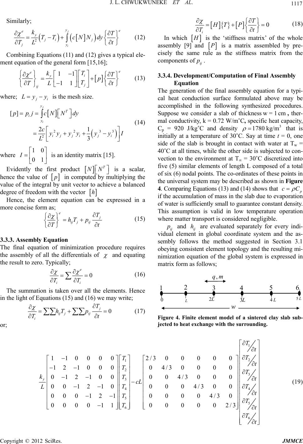

J. L. CHWUKWUNEKE ET AL.
1117
Similarly;



2
j
i
ye
e
y
ji j
jy
kT
TT cNNdy
T L
 

 


t
(12)



0
i
T
HT P
Tt










(18)
In which


H
is the ‘stiffness matrix’ of the whole
assembly [9] and


P is a matrix assembled by pre-
cisely the same rule as the stiffness matrix from the
components of.
ij
p
Combining Equations (11) and (12) gives a typical ele-
ment equation of the general form [15,16];

11
11
e
ei
y
j
ij
T kT
p
T
TL t


 



  





 


(13) 3.3.4. Development/Computati on of Final Assembly
Equation
where;
j
i
Ly y is the mesh size.


22 33
2
[]
21
3
j
i
y
T
i
y
ij jiji
ppjcNNdy
cyyyyyyI
L

 










(14)
The generation of the final assembly equation for a typi-
cal heat conduction surface formulated above may be
accomplished in the following synthesized procedures.
Suppose we consider a slab of thickness, ther-
mal conductivity, k = 0.72 W/m˚C, specific heat capacity,
Cp = 920 J/kg˚C and density that is
initially at a temperature of 30˚C. Say at time t = 0, one
side of the slab is brought in contact with water at Tw =
40˚C at all times, while the other side is subjected to con-
vection to the environment at T∞ = 30˚C discretized into
five (5) similar elements of length L composed of a total
of six (6) nodal points. The co-ordinates of these points in
the universal system may be described as shown in Figure
4. Comparing Equations (13) and (14) shows that p
w = 1cm
3
780 kg/m1  
cC


if the accumulation of mass in the slab due to evaporation
of water is sufficiently small to guarantee constant density.
This assumption is valid in low temperature operation
where matter transport is considered negligible.
where is an identity matrix [15].
10
01
I 

Evidently the first product


T
NN

 
is a scalar,
hence the value of


p in computed by multiplying the
value of the integral by unit vector to achieve a balanced
degree of freedom with the vector


h
Hence, the element equation can be expressed in a
more concise form as;
e
j
ij jij
T
hT p
Tt







 (15)
ij and ij
h are evaluated separately for every indi-
vidual element in global coordinate system and the as-
sembly follows the method suggested in Section 3.1
obeying consistent element topology and the resulting mi-
nimization equation of the global system is expressed in
matrix form as follows;
p
3.3.3. Assembly Equation
The final equation of minimization procedure requires
the assembly of all the differentials of

and equating
the result to zero. Typically;
0
e
ii
TT

 




(16)
The summation is taken over all the elements. Hence
in the light of Equations (15) and (16) we may write;
0
j
ij jij
i
T
hT p
Tt




 

(17)
0
L
L
2
L
3
L
4L5
123456
w
mq,
Figure 4. Finite element model of a sintered clay slab sub-
jected to heat exchange with the sur rounding.
or;
1
2
1
2
3
3
44
5
5
6
110000 2/300000
121000 04/30000
012100004/3000
001210 0004/300
000121 00004/30
000011 000002/3
y
T
t
T
T
t
TT
kTt
cL
TT
L
t
TT
Tt
T



 
 
 
 


 

  

 
 


 

 

 











6t


















(19)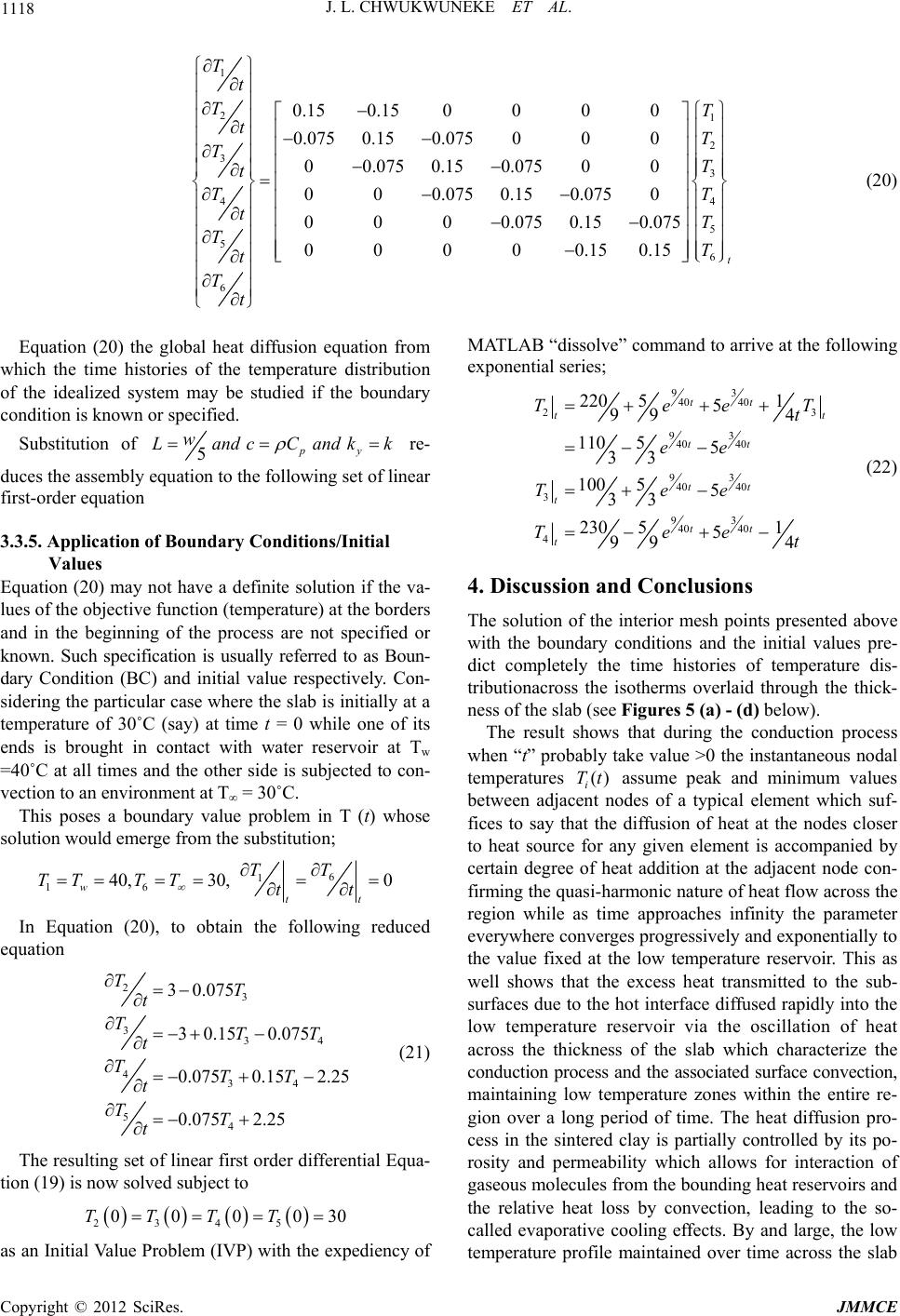

J. L. CHWUKWUNEKE ET AL.
1118
1
21
2
3
3
4 4
5
5
6
6
0.150.1500 0 0
0.075 0.150.075000
00.075 0.150.07500
000.075 0.150.0750
0 0 00.0750.150.075
00000.150.15
T
t
TT
tT
TT
t
T T
tT
TT
t
T
t









  


 




 

 

 

 

 






t











(20)
Equation (20) the global heat diffusion equation from
which the time histories of the temperature distribution
of the idealized system may be studied if the boundary
condition is known or specified.
Substitution of 5py
w
Land cCand kk    re-
duces the assembly equation to the following set of linear
first-order equation
3.3.5. Application of Boundary Conditions/Initial
Values
Equation (20) may not have a definite solution if the va-
lues of the objective function (temperature) at the borders
and in the beginning of the process are not specified or
known. Such specification is usually referred to as Boun-
dary Condition (BC) and initial value respectively. Con-
sidering the particular case where the slab is initially at a
temperature of 30˚C (say) at time t = 0 while one of its
ends is brought in contact with water reservoir at Tw
=40˚C at all times and the other side is subjected to con-
vection to an environment at T∞ = 30˚C.
This poses a boundary value problem in T (t) whose
solution would emerge from the substitution;
6 1
16
40, 30,0
w
tt
T T
TT TTtt

 
 

In Equation (20), to obtain the following reduced
equation
23
334
434
54
3 0.075
3 0.150.075
0.075 0.152.25
0.075 2.25
TT
t
TTT
t
TTT
t
TT
t


 

 

 

(21)
The resulting set of linear first order differential Equa-
tion (19) is now solved subject to



2345
0000 TTTT30
as an Initial Value Problem (IVP) with the expediency of
MATLAB “dissolve” command to arrive at the following
exponential series;
93
40 40
23
93
40 40
93
40 40
3
93
40 40
4
220 51
5
99 4
110 55
33
100 55
33
230 51
5
994
tt
tt
tt
tt
t
tt
t
Tee
t
ee
Tee
Tee
t
 
 

 
T
(22)
4. Discussion and Conclusions
The solution of the interior mesh points presented above
with the boundary conditions and the initial values pre-
dict completely the time histories of temperature dis-
tributionacross the isotherms overlaid through the thick-
ness of the slab (see Figures 5 (a) - (d) below).
The result shows that during the conduction process
when “t” probably take value >0 the instantaneous nodal
temperatures assume peak and minimum values
between adjacent nodes of a typical element which suf-
fices to say that the diffusion of heat at the nodes closer
to heat source for any given element is accompanied by
certain degree of heat addition at the adjacent node con-
firming the quasi-harmonic nature of heat flow across the
region while as time approaches infinity the parameter
everywhere converges progressively and exponentially to
the value fixed at the low temperature reservoir. This as
well shows that the excess heat transmitted to the sub-
surfaces due to the hot interface diffused rapidly into the
low temperature reservoir via the oscillation of heat
across the thickness of the slab which characterize the
conduction process and the associated surface convection,
maintaining low temperature zones within the entire re-
gion over a long period of time. The heat diffusion pro-
cess in the sintered clay is partially controlled by its po-
rosity and permeability which allows for interaction of
gaseous molecules from the bounding heat reservoirs and
the relative heat loss by convection, leading to the so-
called evaporative cooling effects. By and large, the low
temperature profile maintained over time across the slab
()
i
Tt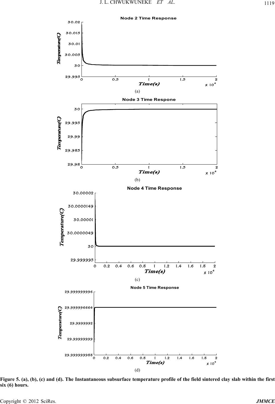

J. L. CHWUKWUNEKE ET AL. 1119
00.5 11.5 2
x 10
4
29.9 9 5
30
30.005
30.01
30.015
30.02
Time(s)
Temperat ure(C
)
Node 2 Ti m e Response
(a)
00.5 11.5 2
x 10
4
29.98
29.9 8 5
29.99
29.995
30
Time(s)
Temperature(C
)
Node 3 Tim e Re sp one
(b)
00.2 0.4 0.6 0.811.2 1.41.6 1.8 2
x 10
4
29.999995
30
30.0000049
30.0 0001
30.0000149
30.00002
Time(s)
Temperat ure( C
)
Node 4 Ti m e Respons e
(c)
00.20.4 0.6 0.8 11.2 1.4 1.61.8 2
x 10
4
29.999999988
29.99999999
29.9999992
29.999996664
29.999999996
Time( s)
Temperat ure(C
)
Node 5 Time Response
(d)
Figure 5. (a), (b), (c) and (d). The Instantaneous subsurface temperature profile of the field sintered clay slab within the first
six (6) hours.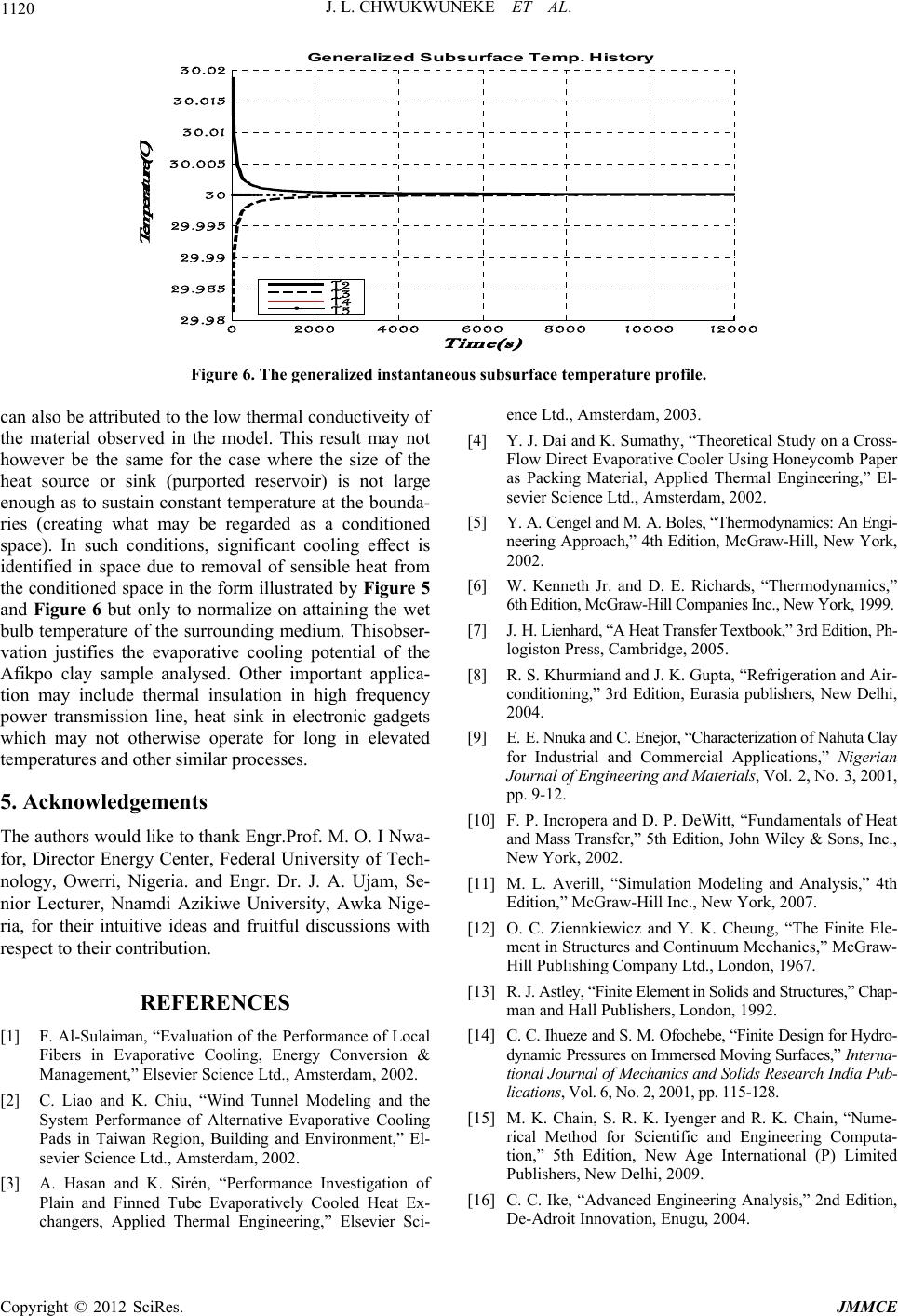

J. L. CHWUKWUNEKE ET AL.
1120
02000 4000 6000 8000 10000 12000
29.98
29.9 85
29.99
29.9 95
30
30.005
30.01
30.015
30.02
Time(s)
Temperature(
C)
G ener al ized Subsurfac e Tem p. Hi st or y
T2
T3
T4
T5
Figure 6. The generalized instantaneous subsurface temperature profile.
can also be attributed to the low thermal conductiveity of
the material observed in the model. This result may not
however be the same for the case where the size of the
heat source or sink (purported reservoir) is not large
enough as to sustain constant temperature at the bounda-
ries (creating what may be regarded as a conditioned
space). In such conditions, significant cooling effect is
identified in space due to removal of sensible heat from
the conditioned space in the form illustrated by Figure 5
and Figure 6 but only to normalize on attaining the wet
bulb temperature of the surrounding medium. Thisobser-
vation justifies the evaporative cooling potential of the
Afikpo clay sample analysed. Other important applica-
tion may include thermal insulation in high frequency
power transmission line, heat sink in electronic gadgets
which may not otherwise operate for long in elevated
temperatures and other similar processes.
5. Acknowledgements
The authors would like to thank Engr.Prof. M. O. I Nwa-
for, Director Energy Center, Federal University of Tech-
nology, Owerri, Nigeria. and Engr. Dr. J. A. Ujam, Se-
nior Lecturer, Nnamdi Azikiwe University, Awka Nige-
ria, for their intuitive ideas and fruitful discussions with
respect to their contribution.
REFERENCES
[1] F. Al-Sulaiman, “Evaluation of the Performance of Local
Fibers in Evaporative Cooling, Energy Conversion &
Management,” Elsevier Science Ltd., Amsterdam, 2002.
[2] C. Liao and K. Chiu, “Wind Tunnel Modeling and the
System Performance of Alternative Evaporative Cooling
Pads in Taiwan Region, Building and Environment,” El-
sevier Science Ltd., Amsterdam, 2002.
[3] A. Hasan and K. Sirén, “Performance Investigation of
Plain and Finned Tube Evaporatively Cooled Heat Ex-
changers, Applied Thermal Engineering,” Elsevier Sci-
ence Ltd., Amsterdam, 2003.
[4] Y. J. Dai and K. Sumathy, “Theoretical Study on a Cross-
Flow Direct Evaporative Cooler Using Honeycomb Paper
as Packing Material, Applied Thermal Engineering,” El-
sevier Science Ltd., Amsterdam, 2002.
[5] Y. A. Cengel and M. A. Boles, “Thermodynamics: An Engi-
neering Approach,” 4th Edition, McGraw-Hill, New York,
2002.
[6] W. Kenneth Jr. and D. E. Richards, “Thermodynamics,”
6th Edition, McGraw-Hill Companies Inc., New York, 1999.
[7] J. H. Lienhard, “A Heat Transfer Textbook,” 3rd Edition, Ph-
logiston Press, Cambridge, 2005.
[8] R. S. Khurmiand and J. K. Gupta, “Refrigeration and Air-
conditioning,” 3rd Edition, Eurasia publishers, New Delhi,
2004.
[9] E. E. Nnuka and C. Enejor, “Characterization of Nahuta Clay
for Industrial and Commercial Applications,” Nigerian
Journal of Engineering and Materials, Vol. 2, No. 3, 2001,
pp. 9-12.
[10] F. P. Incropera and D. P. DeWitt, “Fundamentals of Heat
and Mass Transfer,” 5th Edition, John Wiley & Sons, Inc.,
New York, 2002.
[11] M. L. Averill, “Simulation Modeling and Analysis,” 4th
Edition,” McGraw-Hill Inc., New York, 2007.
[12] O. C. Ziennkiewicz and Y. K. Cheung, “The Finite Ele-
ment in Structures and Continuum Mechanics,” McGraw-
Hill Publishing Company Ltd., London, 1967.
[13] R. J. Astley, “Finite Element in Solids and Structures,” Chap-
man and Hall Publishers, London, 1992.
[14] C. C. Ihueze and S. M. Ofochebe, “Finite Design for Hydro-
dynamic Pressures on Immersed Moving Surfaces,” Interna-
tional Journal of Mechanics and Solids Research India Pub-
lications, Vol. 6, No. 2, 2001, pp. 115-128.
[15] M. K. Chain, S. R. K. Iyenger and R. K. Chain, “Nume-
rical Method for Scientific and Engineering Computa-
tion,” 5th Edition, New Age International (P) Limited
Publishers, New Delhi, 2009.
[16] C. C. Ike, “Advanced Engineering Analysis,” 2nd Edition,
De-Adroit Innovation, Enugu, 2004.