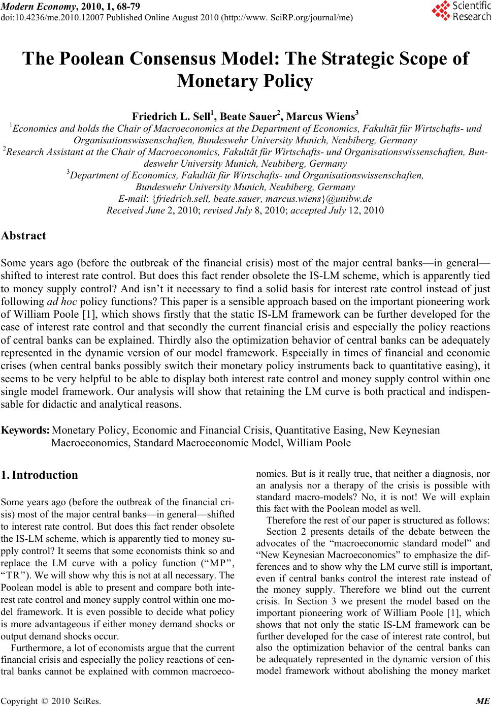Modern Economy, 2010, 1, 68-79
doi:10.4236/me.2010.12007 Published Online August 2010 (http://www. SciRP.org/journal/me)
The Poolean Consensus Model: The Strategic Scope of
Monetary Policy
Friedrich L. Sell1, Beate Sauer2, Marcus Wiens3
1Economics and holds the Chair of Macroeconomics at the Department of Economics, Fakultät für Wirtschafts- und
Organisationswissenschaften, Bundeswehr University Munich, Neubiberg, Germany
2Research Assistant at the Chair of Macroeconomics, Fakultät für Wirtschafts- und Organisationswissenschaften, Bun-
deswehr University Munich, Neubiberg, Germany
3Department of Economics, Fakultät für Wirtschafts- und Organisationswissenschaften,
Bundeswehr University Munich, Neubiberg, Germany
Received June 2, 2010; revised July 8, 2010; accepted July 12, 2010
Abstract
Some years ago (before the outbreak of the financial crisis) most of the major central banks—in general—
shifted to interest rate control. But does this fact render obsolete the IS-LM scheme, which is apparently tied
to money supply control? And isn’t it necessary to find a solid basis for interest rate control instead of just
following ad hoc policy functions? This paper is a sensible approach based on the important pioneering work
of William Poole [1], which shows firstly that the static IS-LM framework can be further developed for the
case of interest rate control and that secondly the current financial crisis and especially the policy reactions
of central banks can be explained. Thirdly also the optimization behavior of central banks can be adequately
represented in the dynamic version of our model framework. Especially in times of financial and economic
crises (when central banks possibly switch their monetary policy instruments back to quantitative easing), it
seems to be very helpful to be able to display both interest rate control and money supply control within one
single model framework. Our analysis will show that retaining the LM curve is both practical and indispen-
sable for didactic and analytical reasons.
Keywords: Monetary Policy, Economic and Financial Crisis, Quantitative Easing, New Keynesian
Macroeconomics, Standard Macroeconomic Model, William Poole
1. Introduction
Some years ago (before the outbreak of the financial cri-
sis) most of the major central banks—in general—shifted
to interest rate control. But does this fact render obsolete
the IS-LM scheme, which is apparently tied to money su-
pply control? It seems that some economists think so and
replace the LM curve with a policy function (“MP”,
“TR”). We will show why this is not at all necessary. The
Poolean model is able to present and compare both inte-
rest rate control and money supply control within one mo-
del framework. It is even possible to decide what policy
is more advantageous if either money demand shocks or
output demand shocks occur.
Furthermore, a lot of economists argue that the current
financial crisis and especially the policy reactions of cen-
tral banks cannot be explained with common macroeco-
nomics. But is it really true, that neither a diagnosis, nor
an analysis nor a therapy of the crisis is possible with
standard macro-models? No, it is not! We will explain
this fact with the Poolean model as well.
Therefore the rest of our paper is structured as follows:
Section 2 presents details of the debate between the
advocates of the “macroeconomic standard model” and
“New Keynesian Macroeconomics” to emphasize the dif-
ferences and to show why the LM curve still is important,
even if central banks control the interest rate instead of
the money supply. Therefore we blind out the current
crisis. In Section 3 we present the model based on the
important pioneering work of William Poole [1], which
shows that not only the static IS-LM framework can be
further developed for the case of interest rate control, but
also the optimization behavior of the central banks can
be adequately represented in the dynamic version of this
model framework without abolishing the money market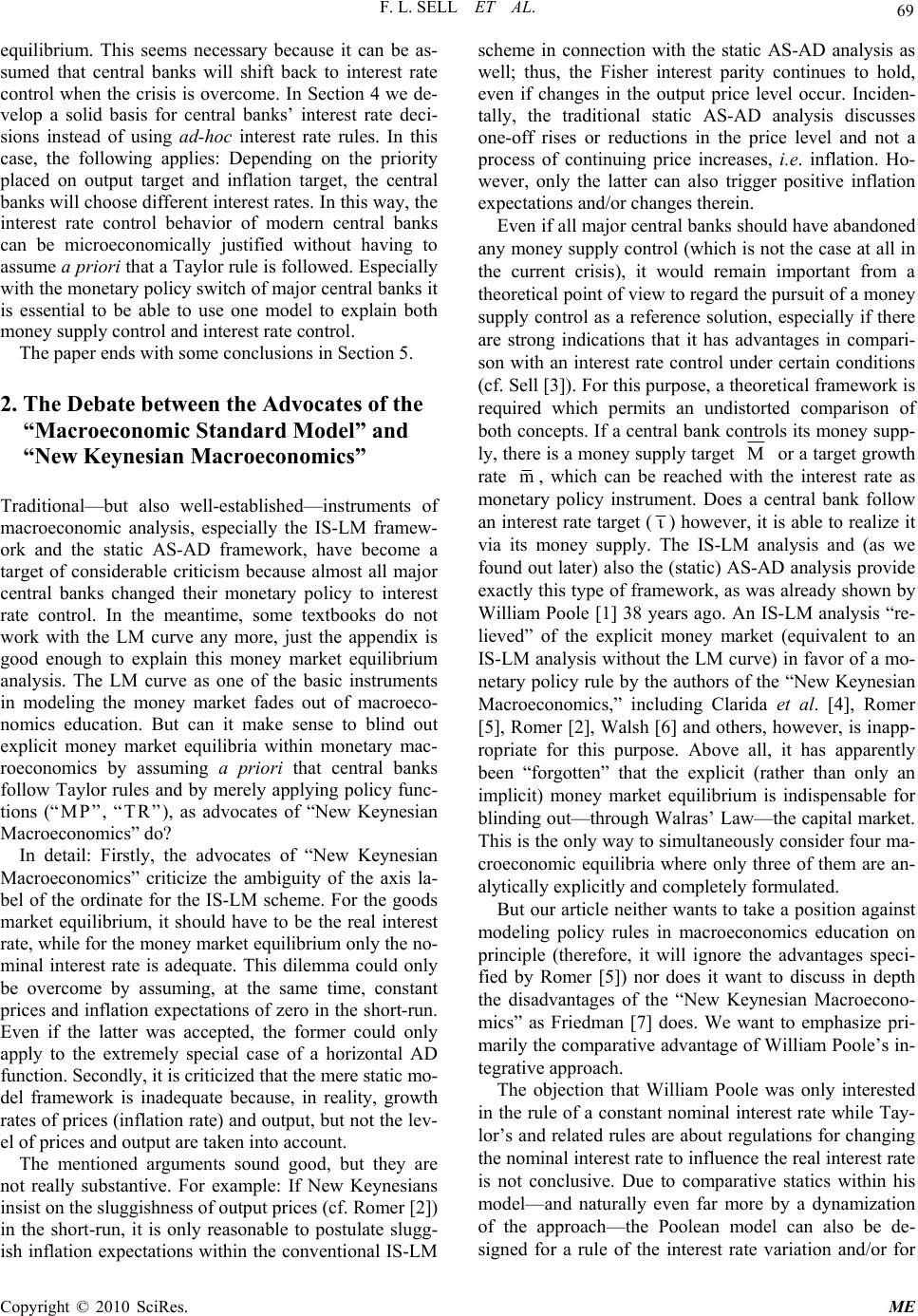

F. L. SELL ET AL.
69
equilibrium. This seems necessary because it can be as-
sumed that central banks will shift back to interest rate
control when the crisis is overcome. In Section 4 we de-
velop a solid basis for central banks’ interest rate deci-
sions instead of using ad-hoc interest rate rules. In this
case, the following applies: Depending on the priority
placed on output target and inflation target, the central
banks will choose different interest rates. In this way, the
interest rate control behavior of modern central banks
can be microeconomically justified without having to
assume a priori that a Taylor rule is followed. Especially
with the monetary policy switch of major central banks it
is essential to be able to use one model to explain both
money supply control and interest rate control.
The paper ends with some conclusions in Section 5.
2. The Debate between the Advocates of the
“Macroeconomic Standard Model” and
“New Keynesian Macroeconomics”
Traditional—but also well-established—instruments of
macroeconomic analysis, especially the IS-LM framew-
ork and the static AS-AD framework, have become a
target of considerable criticism because almost all major
central banks changed their monetary policy to interest
rate control. In the meantime, some textbooks do not
work with the LM curve any more, just the appendix is
good enough to explain this money market equilibrium
analysis. The LM curve as one of the basic instruments
in modeling the money market fades out of macroeco-
nomics education. But can it make sense to blind out
explicit money market equilibria within monetary mac-
roeconomics by assuming a priori that central banks
follow Taylor rules and by merely applying policy func-
tions (“MP”, “TR”), as advocates of “New Keynesian
Macroeconomics” do?
In detail: Firstly, the advocates of “New Keynesian
Macroeconomics” criticize the ambiguity of the axis la-
bel of the ordinate for the IS-LM scheme. For the goods
market equilibrium, it should have to be the real interest
rate, while for the money market equilibrium only the no-
minal interest rate is adequate. This dilemma could only
be overcome by assuming, at the same time, constant
prices and inflation expectations of zero in the short-run.
Even if the latter was accepted, the former could only
apply to the extremely special case of a horizontal AD
function. Secondly, it is criticized that the mere static mo-
del framework is inadequate because, in reality, growth
rates of prices (inflation rate) and output, but not the lev-
el of prices and output are taken into account.
The mentioned arguments sound good, but they are
not really substantive. For example: If New Keynesians
insist on the sluggishness of output prices (cf. Romer [2])
in the short-run, it is only reasonable to postulate slugg-
ish inflation expectations within the conventional IS-LM
scheme in connection with the static AS-AD analysis as
well; thus, the Fisher interest parity continues to hold,
even if changes in the output price level occur. Inciden-
tally, the traditional static AS-AD analysis discusses
one-off rises or reductions in the price level and not a
process of continuing price increases, i.e. inflation. Ho-
wever, only the latter can also trigger positive inflation
expectations and/or changes therein.
Even if all major central banks should have abandoned
any money supply control (which is not the case at all in
the current crisis), it would remain important from a
theoretical point of view to regard the pursuit of a money
supply control as a reference solution, especially if there
are strong indications that it has advantages in compari-
son with an interest rate control under certain conditions
(cf. Sell [3]). For this purpose, a theoretical framework is
required which permits an undistorted comparison of
both concepts. If a central bank controls its money supp-
ly, there is a money supply target M or a target growth
rate m, which can be reached with the interest rate as
monetary policy instrument. Does a central bank follow
an interest rate target (

) however, it is able to realize it
via its money supply. The IS-LM analysis and (as we
found out later) also the (static) AS-AD analysis provide
exactly this type of framework, as was already shown by
William Poole [1] 38 years ago. An IS-LM analysis “re-
lieved” of the explicit money market (equivalent to an
IS-LM analysis without the LM curve) in favor of a mo-
netary policy rule by the authors of the “New Keynesian
Macroeconomics,” including Clarida et al. [4], Romer
[5], Romer [2], Walsh [6] and others, however, is inapp-
ropriate for this purpose. Above all, it has apparently
been “forgotten” that the explicit (rather than only an
implicit) money market equilibrium is indispensable for
blinding out—through Walras’ Law—the capital market.
This is the only way to simultaneously consider four ma-
croeconomic equilibria where only three of them are an-
alytically explicitly and completely formulated.
But our article neither wants to take a position against
modeling policy rules in macroeconomics education on
principle (therefore, it will ignore the advantages speci-
fied by Romer [5]) nor does it want to discuss in depth
the disadvantages of the “New Keynesian Macroecono-
mics” as Friedman [7] does. We want to emphasize pri-
marily the comparative advantage of William Poole’s in-
tegrative approach.
The objection that William Poole was only interested
in the rule of a constant nominal interest rate while Tay-
lor’s and related rules are about regulations for changing
the nominal interest rate to influence the real interest rate
is not conclusive. Due to comparative statics within his
model—and naturally even far more by a dynamization
of the approach—the Poolean model can also be de-
signed for a rule of the interest rate variation and/or for

F. L. SELL ET AL.
70
change rates of the price level and of the output. Espec-
ially if the conviction prevails that modern central banks
do not (or no longer) pursue any money supply control,
but interest rate control (it really was the case until the
start of the economic crisis in 2008 and most likely it
will be the case again after the crisis), it appears outright
bizarre to associate the European Central Bank’s (ECB)
or US-Fed’s monetary policy with a Taylor rule as an ex-
ante strategy in the new millennium. The ECB largely co
ncentrates on stabilizing the price level while the Federal
Reserve has already stepped in for the second time since
2001 to contain damage during and after a financial mar-
ket crisis. Therefore a Poolean interest rate control seems
to be appropriate in a twofold way: Not only does it re-
tain the concept of the explicit money market equilibri-
um, it can also be oriented contractively or expansively
depending on the requirements, irrespective of whether
the acting central bank is committed exclusively to the
aim of price level stability or also to the overall econom-
ic output and/or the aim of creating employment.
3. The Static Poolean Consensus Model in
the Short-Run
Figure 1 shows a simple money market in which the
“traditional” money supply control of central banks can
be described: With a short-run (sluggish) output price
level (P0), the central bank aims at the (nominal) money
supply target M; for this purpose, interest rate level i
is a suitable means. If fluctuations in the money demand
—due to increases in income (Y) or shocks (u) —occur
between L0 and L1 and/or L2 then the central bank will
continue to reach its target money supply by adapting the
(hence endogenous) interest rate level to the new amount
i1 and/or i2.
In Figure 2, we can describe the interest rate control
conducted by central banks in accordance with Poole
(1970): In order to achieve the desired interest rate i, the
central bank must—for a specific money demand L0
—now provide money supply M0. If fluctuations in the
money demand occur between L0 and L1 and/or L2 (for
similar reasons as described above), then the central bank
would have to adjust the money supply toward level

1
M
and/or

2 M. On the other hand, the central bank is still
able to adapt its key interest rate to a changed environ-
ment and adopt a more expansive (contractive) policy.
For a target interest rate of i1 (i2) it must stear the money
supply toward level M1 (M2). Interest rate control and
money supply control exhibit different comparative ad-
vantages: Interest rate control proves especially favor-
able if money demand shocks occur. These are not un-
common during the introduction of a currency union.
That is why in 1999 the ECB gave priority to an interest
rate control in contrast to the money supply control of
the Deutsche Bundesbank. Already in the 1970s William
Poole showed the comparative advantages of that policy
compared to money supply control when money demand
shocks occur.
Figure 1. Money supply control according to W. Poole (1970).

F. L. SELL ET AL.
71
As shown in Figure 3, the pursuit of interest rate con-
trol permits, as a general rule, to completely prevent po-
tential output fluctuations (LM3 (i)), while the pursuit of
money supply control cannot prevent shifts of the LM
curve (LM1 and/or LM2); thus corresponding output
fluctuations in interval Y1 – Y2 have to be accepted.
The comparative advantages show a completely diff-
erent distribution when shocks to the output demand dis-
turb the initial equilibrium: As demonstrated in Figure 4,
the pursuit of money supply control reduces the potential
output fluctuations to interval Y3 – Y4, while the orienta-
tion of the monetary policy towards interest rate control
extends the interval to the new limits Y5 – Y6, which
signify a much larger output fluctuation.
Figure 2. Interest rate control according to W. Poole (1970).
Figure 3. Output stabilization in the case of money demand shocks according to W. Poole (1970).

F. L. SELL ET AL.
72
Figure 4. Output stabilization in the case of output demand shocks according to W. Poole (1970).
The current crisis is nothing other than an output de-
mand shock where money supply control is more advan-
tageous. All major central banks followed Poole’s rec-
ommendation and shifted away from interest rate control
to quantitative easing. To avoid a so-called zero-interest-
rate-policy, the US-Fed and the Bank of England chang-
ed their instruments when reaching the 0.25 and 0.5 per-
cent threshold, respectively. Because of the blocked tra-
nsmission channel (reduction of the key interest rate is
not passed through to private economic agents by comm-
ercial banks/does not lead to lower interest rates on mon-
ey markets), both central banks bought government sec-
urities and/or toxic assets to expand the monetary basis
via money printing. This quantitative easing cannot be
demonstrated without the LM curve. When the effects of
the current financial crisis will be overcome, interest rate
control is again conceivable as the adequate monetary
policy instrument.
The effectiveness of monetary and fiscal policies can
be examined in conjunction with the static AS-AD sc-
heme (as it is described in Blanchard [8]) without aband-
oning the LM curve, where the central bank pursues—in
the sense of Poole, but also in the sense of the “New Ke-
ynesian Macroeconomics”—interest rate control in an
endogenous money supply environment.
We will take the following, strongly simplified struc-
ture as the basis model:
Let Y be the output of the economy, Aa the domestic
autonomous absorption, h the marginal propensity to
invest and r the real interest rate. Then the IS curve takes
the common form

a
YAhr  , (1)
where 1
1cct


, with c being the marginal propen-
sity to consume and t being the rate of taxation.
The money market is represented by the LM curve

1
ikYMu
j


, (2)
with i denoting the nominal interest rate, k the transac-
tion motive of the money demand, j the speculation mo-
tive of the money demand, M the real money supply, and
where u is a shock term distributed with zero mean and
variance 2

.
The real money supply is defined as
n
M
MP , (3)
where n
M
is the nominal money supply and P stands
for the price level.
The central bank’s nominal interest rate control can be
written as:
ii


(4)
The right-hand side of Equation (4) replaces the right-
hand side of the LM curve, because the central bank
compensates for fluctuations in the money demand as a
consequence of income changes and/or under the influ-
ence of shocks in such a way that its interest rate concept
materializes. As no distinction is made between the nomi-
nal and the real interest rates within the short-run (i = r),
i* can directly be inserted in the IS curve (1):


a
YAhi

  (5)

F. L. SELL ET AL.
73
Thus, the AD curve generated runs vertically and is
therefore completely price inelastic. In the case of an
increase (a reduction) in the interest rate, it shifts in a
parallel manner to the left (right):
0
Yh
i
 
 (6)
In conjunction with a very simple AS function (cf. Do-
rnbusch/Fischer [9])

11nat
PP YY



, (7)
with γ as a weighting coefficient and Ynat as the natural
output level, a compact AS-AD scheme can be obtained
in the case of interest rate control, but without abandon-
ing the money market equilibrium concept.
An expansive (contractive) monetary policy (Figure 5)
determines a lower (higher) interest rate compared to the
initial level i0, which causes the entire LM curve to shift
down (up) to the new interest rate level i1(i2). In the ag-
gregated supply and demand chart, the monetary policy
results in an excess demand in the amount of Y1 – Y0
(excess supply in the amount of Y0 – Y2) for the initial
price level P0 because of the short-run sluggishness of
prices. The subsequent price increase to P1 (price reduc-
tion to P2) lowers (raises) the value of the real money
supply and/or the equally high real balance. As a conse-
quence (in the medium-run), interest rates will rise to i′1
(fall to i′2), provided the central bank does not compen-
sate for this effect. In both cases, the desired higher in-
come/higher price level (lower income/reduced price
level) will be achieved.
Figure 5. Expansive/contractive monetary policy in the case of interest rate control.

F. L. SELL ET AL.
74
Finally, in Figure 6, the options of fiscal policy are
discussed for the case of interest rate control. An expan-
sive (contractive) fiscal policy creates (analogous with
the above) an excess demand (excess supply) in the ag-
gregated supply and demand chart for the initial price
level P0. The subsequent price increase (price reduction)
lowers (raises) the value of the real money supply and/or
the equally high real balance. As a consequence (in the
medium-run), interest rates will also rise to i1 (fall to i2)
and the LM curve will shift up (down) accordingly, again
provided the central bank does not compensate for this
effect. In both cases fiscal policy now achieves the de-
sired higher income/higher price level (lower income/
reduced price level).
By the way, it is possible to add the upward sloping
Fleming-Mundell ZZ curve to the existing description
and, hence, to shift to the open economy very easily (cf.
Sell [3]). The use of Poole’s approach in an open econ-
omy case to explain and compare the different central
bank policies is doable as well. Sell/Kermer [10] did a
formal analysis of possible losses caused by either a coo-
perative or a non-cooperative strategy when designing
interest rate control or money supply control in open ec-
onomies.
4. A General Derivation of a Central Bank`s
Optimal Interest Rate Policy
In the aftermath of the current financial crisis the central
banks will probably switch back to interest rate control
(see above). Therefore, in the meantime, it is very impo-
rtant to develop a decision logical and solid basis to exp-
lain interest rate control instead of using ad hoc interest
rate rules like the Taylor rule. Such an optimization app-
roach for central banks is described below.
Figure 6. Expansive/contractive fiscal policy in the case of interest rate control.

F. L. SELL ET AL.
75
What is rarely noticed is that Poole [1] (pp. 204 ff.), in
his much-noticed contribution, already worked success-
fully with the instrument of an overall economic welfare
loss function. In this context, he minimized the expected
value of the squared deviation between the current output
and the target output (output gap) with regard to applying
interest rates as a policy instrument and, alternatively,
with regard to money supply control.
If the central bank chooses the nominal interest rate as
the “operating target”, then it has direct influence on the
real output given the equilibrium condition for the goods
market. If, for the medium-run, the real interest rate in
the IS curve (r) is replaced by the nominal interest rate
and inflation expectations (e ) in accordance with the
Fisher interest rate parity (e ri

 ), and the nominal
interest rate is replaced by the interest rate target (see
Equation (4)), the following is obtained:

e
a
YAhhi

  (8)
In the case of given autonomous absorption and given
inflation expectations, an exogenous interest rate reduc-
tion (increase) leads to a rising (falling) real output. This
real output level Y determines, in turn, the inflation rate,
as can easily be seen from the dynamized AS function
(cf. Dornbusch/Fischer [9]):

nat e
YY (9)
If income increases, inflation also rises c. p. (i.e. with
an unchanged level of the natural output) within the same
period.
If the central bank pursues interest rate control, it infl-
uences the output via the correlation of the IS curve (Eq-
uation (8)) and, in a second step, the level of inflation via
the correlation of the AS curve. The transmission chann-
els of monetary policy can be directly derived by insert-
ing Equation (8), the medium-run IS curve, into (9), the
dynamized AS curve:

()1 e nat
a
iAhY hi    (10)
The lower (higher) the interest rate is, the higher (lo-
wer) the inflation rate will be—for a given autonomous
absorption, given inflation expectations, and a given na-
tural output level. Accordingly, it is easier for the central
bank to achieve a low inflation rate, the lower the infla-
tion expectations are and the higher the natural output
level is.
The central bank now minimizes a welfare loss func-
tion L by solving the following problem:
min
iL where
 

2
2
[,] 1nat LiYi YY
, (11)
and  denotes a weighting coefficient,  an external-
ity.
The central bank will thus choose an interest rate to
minimize the welfare losses due to inflation and output
fluctuations. For simplification, the target inflation rate
will be determined to be equal to zero. The output target
envisaged by the central bank corresponds to the natural
output Ynat plus an externality . The latter reflects the
usual assumption of some frictions due to taxes, imper-
fect competition etc. The central bank then tries to over-
come these inefficiencies by a higher output target. The
specific interest rate i* which minimizes the welfare
losses (for an overview of optimizing approaches to gain
policy rules cf. Walsh [11]) is given by:



2
2
11
11
1
1
nat
a
e
iA Y
hh
hh
hh











 








 


(12)
If we take Equations (12) and (10) together, we get the
optimal inflation rate:



2
1
,1
ee
i
 

 





(13)
The most significant determinants of the inflation rate
are inflation expectations and the externality. Both para-
meters have a positive impact on inflation.
Any optimal inflation level which satisfies Equation
(13) is basically feasible. However, we should account
for rational expectations as a standard consistency requ-
irement of any model with forward looking behavior. In
line with the well-known Lucas critics it is common pra-
ctice to interpret the equilibrium under rational expecta-
tions as the long-run outcome of the economy and thus
as a state where policy measures are ineffective since an-
ticipation errors no longer occur. To find out the optimal
inflation rate under rational expectations we simply add
the condition e

 to (13) and get:



1
i


 (14)
Figure 7 is an illustration of the rational expectation
equilibria. The equilibria are all points where our optimal
inflation function


,e i

 crosses the dashed bisecting
line (e

 ).
The plot contains three different values for the wei-
ghting coefficient θ: The upper bound θ = 1 (priority
exclusively on fighting inflation), the lower bound θ = 0
(priority exclusively on preventing output fluctuations),
and an intermediate value for θ. As we can see, for θ = 1
the inflation function becomes horizontal, which leads to
the null inflation equilibrium. As the central bank has the
highest possible preference for price stability, the audi-

F. L. SELL ET AL.
76
ence is convinced enough to believe it (0
e
 ).
With smaller θ, both intercept and slope of the inflation
function rise, which lead to higher inflation rates (and
expected inflation rates respectively) in equilibrium. For
θ = 0 we get a somewhat extreme result: Both functions
run in parallel, which means that they never intersect:
The limit θ → 0 implies that inflation and expectations
together build up to infinity: e

 . In this case,
the central bank completely ignores price stability and
just concentrates on output stabilization. The audience
takes this total neglect into account and expects an ex-
treme inflation path.
If we take Equations (8) and (12) together, we get the
optimal output level:
 

2
,1
e
e nat
Yi Y
 
 

  (15)
The natural level Ynat represents the benchmark of
output fluctuations. Further important parameters deter-
mining the optimal output level are again inflation ex-
pectations and the externality. However, each of the two
influences output by a different sign: The impact of the
externality on output is positive which should be quite
clear since ∆ is a positive externality and the central bank
tries to adjust upwards (if θ < 1). Higher inflation expec-
tations however curtail the output level, since a rising πe
comes with a higher interest rate.
To provide some benchmark solutions we now calcu-
late the optimal interest rate i*, the optimal inflation rate
π* and the optimal output level Y* for the extreme con-
stellations of the weighting factor upper bound θ = 1
(priority exclusively on fighting inflation) and lower
bound θ = 0.
For θ = 1, we obtain:
1
11 1
1
nat e
a
iAY
hh h








(16)
For the output and the inflation rate, the values ind-
uced with this interest rate are:
1
1
() nat e Yi Y





and

10i 
. (17)
We obtain these values by inserting Equation (13) into
Equations (8) and (10) respectively for given inflation
expectations. Accordingly, if the central bank places its
priority exclusively on a lower inflation rate, then it will
achieve an inflation rate amounting to zero. However,
the resulting output is—as can be seen from (17)—below
its natural level. For the opposite case θ = 0, we obtain:

1
11
nat e
a
iAY
hh




 (18)
For the output and the inflation rate, the values indu-
ced with this interest rate are:
1
() nat Yi Y



 and

1
e
i



 . (19)
Figure 7. Rational expectation equilibria.

F. L. SELL ET AL.
77
A central bank which exclusively pursues the objec-
tive of preventing deviations from the natural output will
reach this target in the short-run: The output then ex-
ceeds its natural state by the externality ∆. The inflation
rate is clearly positive: Inflation is partly composed of
the central banks’ incentive to overcome the inefficiency
(∆) on the one hand and of inflation expectations on the
other hand (e
). In this scenario, the short-run interest
rate is lower (cf. with expression (16)), because a low
interest rate is the means for extremely expansive mone-
tary policy. Both benchmark solutions discussed so far
are short-run. In the long-run, the strategy of the central
bank will be anticipated by the audience so that the op-
timal interest rate and the output must be in accordance
with the inflation rate under rational expectations


(cf.
Equation (14)). The corresponding output rate is clearly
the natural output level Ynat (for all θ), so in the long-run
the central bank’s effort to compensate the externality
and to push the output beyond the natural level will sim-
ply evaporate. The optimal interest rate is given by:



11
nat
a
iAY
hh
 
 with


1
 
 (20)
Now the model is nearly complete and we add the last
component. The derived values for the inflation rate and
the output must at all time be compatible with the money
market equilibrium (LM curve). This poses no problem,
because the money supply will automatically adapt itself
to changes in the interest rate (triggered by the central
bank). In order to describe this constraint adequately, the
dynamized version of the LM curve (Equation (2)) will
be used (cf. Dornbusch/Fischer [9] and McCallum [12]):

11tt tt
mkYYjii

  (21)
The rate of change in the nominal money supply m
(monetary expansion or contraction) will adapt itself in
such a way that the change in the real money supply
(left-hand side of Equation (20)) corresponds to the
change in the real money demand (right-hand side of
Equation (20)). If we take into account that, in the case
of interest rate control, the variables π und Y result from
Equations (8) and (10) respectively, and if we insert the
optimal interest rate from Equation (12) into Equation
(20), we obtain the change in the nominal money supply
as a function of the weighting coefficient θ. For the two
extreme cases of exclusive priority placed on inflation
containment (θ = 1) and/or to the minimization of output
fluctuations (θ = 0), we obtain for m:
11
1
nat
t
e
at
j
mkYji
h
jjk
AkYj
hh
 


 




 

 

(22)

11
1
1
nat
t
at
e
j
mkYji
h
jj
AkYkj
hh
j
 


 









 
(23)
It can be seen from the last term of both equations that,
in the case of an exclusive inflation target (Equation
(21)), the higher the inflation expectations are, the lower
the monetary expansion will be. In other words, the in-
flation expectations must be “broken” in this case. How-
ever, in the case of an exclusive output target (Equation
(22)), the monetary expansion will rise in step with the
inflation expectations. If the central bank does not pay
any attention to the costs resulting from inflation, the
inflation expectations will merely be “accommodated”.
Figure 8 graphically represents the entire situation in a
(π, Y) chart. In the long-run the equilibrium is character-
ized by rational expectations. In this case the economy
reaches its natural output level Ynat for all levels of (ex-
pected) inflation. The vertical line

() thus represents
the long-run Phillips-Curve.
The set of curves represent indifference curves for
various values of the loss function L. An arbitrary indif-
ference curve with welfare loss L and weighting coef-
ficient θ can easily be determined by rearranging objec-
tive function (11) to π.
 

2 1nat
L
YYY


 
 (24)
A low weighting coefficient (θL) for the inflation tar-
get (e.g. θ = 0.2) corresponds to the set of strongly con-
cave indifference curves. Accordingly θH (e.g. θ = 0.8)
corresponds to weakly concave indifference curves. The
strong concavity for a low priority on inflation can be
explained by the fact that the central bank accepts a rela-
tively high rise in the inflation rate in order to come
somewhat closer to achieving target output Ynat + ∆.
Consequently, for a high priority on inflation, the indif-
ference curves are weakly concave, because in this case
the central bank accepts relatively strong deviations from
the target output in order to achieve a slight reduction in
the inflation rate. The straight lines with negative slope
represent the money market equilibrium condition: They
describe all combinations of inflation rate and income
which are consistent with a specific level of monetary
expansion m. In this context, value mθ = 1 corresponds to
the constellation for θ = 1 (see Equation (21) and point A
in Figure 8) and, consequently, mθ = 0 corresponds to
the constellation for θ = 0 (see Equation (22) and point B
in Figure 8). We obtain the straight line for a specific
weighting coefficient θ by inserting m(θ) together with i*
into Equation (17) and by rearranging to π. In this way,
being a function of the chosen weighting coefficient θ,

F. L. SELL ET AL.
78
Figure 8. Optimal monetary policy in the case of interest rate control.
all (π, Y) combinations achievable by monetary policy
can be described by the straight line with positive slope
AB . This line represents the (short-run) Phillips-Curve.
A situation represented by Equation (17) (θ = 1) can be
found at point A: The inflation rate is zero, but the output
is lower than the natural output. The change in money
supply occurs in a contractive manner. The intercept of
the money market line mθ = 1 is below the inflation ex-
pectations; thus, a contractive monetary policy must
“break” the inflation expectations in order to be able to
achieve the desired zero inflation rate. The situation de-
scribed by Equation (19) (θ = 0) exists at point B: Here
the inflation rate is exactly at the level of the inflation
expectations and, accordingly, also the achieved output is
at its natural level. In this case, the intercept of the mo-
ney market line mθ = 0 is above the inflation expectations.
The output is higher than in the “natural state”: The
money supply will adapt itself in such a way that, first,
the money demand (


nat
kY k) is satisfied and,
second, inflation expectations (πe) are accommodated.
5. Conclusions
The IS-LM framework originating from Keynes’ discip-
les Alvin Hansen and John Hicks can—as has been dem-
onstrated by this contribution—be appropriately ext-
ended to the case of interest rate control conducted by
central banks without having to abandon the equilibrium
concept of the IS-LM analysis, as has been vehemently
maintained by advocates of “New Keynesian Macroeco-
nomics” for years. Especially in times of financial and ec-
onomic crises (when central banks possibly switch their
monetary policy instruments back to quantitative easing),
it seems to be very helpful to be able to display both int-
erest rate control and money supply control within one
single model framework. For a comprehensive—rather
than simply partial—analysis of the macroeconomics of
monetary policy it is objectionable to blind out the mo-
ney market as such. Our analysis has shown that retain-
ing the LM curve is both practical and indispensable for
didactic and analytical reasons.
In addition, it is possible to design the dynamic vers-
ion of the IS-LM framework in such a way that it is com-
patible with the optimization behavior of central banks in
the case of interest rate control and that it provides very
general determining reasons for choosing the key interest
rate instead of following a policy rule.
Finally, it is easy to extend our framework to illustrate
specific problems of optimal monetary policy, e.g. time
inconsistency (cf. Kydland/Prescott [13]).
Our model confirms the impression that macroeco-
nomic analysis should continue to work with a somewhat
generalized and consistent framework—instead of put-
ting aside the LM curve i.e. the explicit money market
equilibrium as done in Graf Lambsdorff/Engelen [14].
6. References
[1] W. Poole, “Optimal Choice of Monetary Policy Instru-
ments in a Simple Stochastic Macro Model,” Quarterly

F. L. SELL ET AL.
79
Journal of Economics, Vol. 84, No. 2, May 1970, pp.
197-216.
[2] D. Romer, “Short-Run Fluctuations,” University of Cali-
fornia, Berkeley, August 2002.
[3] F. L. Sell, “Zins- und Geldmengensteuerung in Der off-
enen Volkswirtschaft,” WISU—Das Wirtschaftsstu- dium,
Vol. 35, No. 3, May 2006, pp. 363-372 and 379-380.
[4] R. Clarida, J. Galí and M. Gertler, “The Science of Mon-
etary Policy: A New Keynesian Perspective,” Journal of
Economic Literature, Vol. 37, No. 4, December 1999, pp.
1661-1707.
[5] D. Romer, “Keynesian Macroeconomics without the LM
Curve,” Journal of Economic Perspectives, Vol. 14, No.
2, Spring 2000, pp. 149-169.
[6] C. E. Walsh, “Teaching Inflation Targeting: An Analysis
for Intermediate Macro”, Journal of Economic Education,
Vol. 33, No. 4, 2002, pp. 333-346.
[7] B. Friedman, “The LM Curve: A Not-So-Fond Farewell,”
NBER Working Paper Series, No. 10123, November 2003.
[8] O. Blanchard, “Macroeconomics,” 4th Edition, Prentice
Hall, 2006.
[9] R. Dornbusch, S. Fischer and R. Startz, “Macroeconom-
ics,” 10th Edition, McGraw-Hill/Irwin, New Delhi, 2007.
[10] F. L. Sell and S. Kermer, “William Poole in der Offenen
Volkswirtschaft,” Kredit und Kapital, Vol. 41, No. 4,
2008, pp. 467-500.
[11] C. E. Walsh, “Monetary Theory and Policy,” 2nd Edition,
The MIT Press, Cambridge, 2003.
[12] B. T. McCallum, “Monetary Economics—Theory and
Policy,” Macmillan Publishing, New York, 1989.
[13] F. E. Kydland and E. C. Prescott, “Rules rather than Dis-
cretion: The Inconsistency of Optimal Plans,” Journal of
Political Economy, Vol. 85, No. 3, April 1977, pp. 473-491.
[14] J. G. Lambsdorff and C. Engelen, “Das Keynesi- anische
Konsensmodell,” Wirtschaftswissenschaft- liches Studium
(WiSt), Vol. 36, No. 7, August 2007, pp. 387-393.