Journal of Modern Physics
Vol.3 No.9A(2012), Article ID:23121,10 pages DOI:10.4236/jmp.2012.329168
A Global Solution of the Einstein-Maxwell Field Equations for Rotating Charged Matter
School of Physics Astronomy and Mathematics, University of Hertfordshire, Hatfield, UK
Email: a.georgiou@herts.ac.uk
Received June 27, 2012; revised July 31, 2012; accepted August 9, 2012
Keywords: Gravitation; Exact Solutions; Einstein-Maxwell Equations; Rotation; Charged Dust
ABSTRACT
A stationary axially symmetric exterior electrovacuum solution of the Einstein-Maxwell field equations was obtained. An interior solution for rotating charged dust with vanishing Lorentz force was also obtained. The two spacetimes are separated by a boundary which is a surface layer with surface stress-energy tensor and surface electric 4-current. The layer is the spherical surface bounding the charged matter. It was further shown, that all the exterior physical quantities vanished at the asymptotic spatial infinity where spacetime was shown to be flat. There are two different sets of junction conditions: the electromagnetic junction conditions, which were expressed in the traditional 3-dimensional form of classical electromagnetic theory; and the considerably more complicated gravitational junction conditions. It was shown that both—the electromagnetic and gravitational junction conditions—were satisfied. The mass, charge and angular momentum were determined from the metric. Exact analytical formulae for the dipole moment and gyromagnetic ratio were also derived. The conditions, under which the latter formulae gave Blackett’s empirical result for rotating stars, were investigated.
1. Introduction
There are difficulties in finding exact solutions of the Einstein or of the Einstein-Maxwell field equations for a volume distribution of rotating bounded matter [1]. Such solutions should consist of an interior filled with matter and an asymptotically flat vacuum or electrovacuum exterior, these being separated by a surface on which appropriate boundary conditions should be satisfied. The main aim of this work is to obtain an exterior and matching interior solution of the Einstein-Maxwell field equations with finite bounded rotating charged matter as a source of the spacetime. Due to the rotation, the boundary will actually be an oblate spheroid, but it is assumed that it is a spherical surface with equation r = a. The main objective and emphasis after all, is to see how far the attempt at finding a solution can be taken—a solution with finite bounded rotating matter as a source of the spacetime. The additional complication of spheroidal coor-dinates is avoided, in a problem which is already enormously complicated.
Most of the equations and expressions for the various physical quantities are difficult to derive and they require involved and lengthy analysis. It is not therefore possible or desirable to include these calculations in the paper, but directions in which to proceed are indicated.
2. The Einstein-Maxwell Field Equations
Consider electrically charged pressure-free matter (charged dust) bounded by the hypersurface r = a and rotating with constant angular velocity about the polar axis  under zero Lorentz force. It is assumed that the current is carried by the dust. The transformed expression (2.1) in [2] for the Weyl-Lewis-Papapetrou metric for a stationary axially symmetric spacetime V is
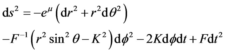 (1)
(1)
where we have taken the signature of the spacetime metric tensor  to be
to be  It is implicit in the form (1) of the metric that we have assumed, without loss of generality, that
 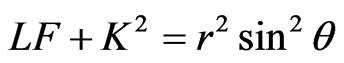 and so the component
  of
of  is
is  We shall use units c = G = 1 where
  is the vacuum speed of light and G the Newtonian gravitational constant. Unless otherwise specified, we shall adopt the convention in which Roman indices take the values 1, 2, 3 for the space coordinates
 which are spherical polar coordinates co-moving with the dust, and Greek indices take the values
  for the spacetime coordinates
 . Semicolons and commas indicate covariant and partial derivatives respectively, and the suffixes r and θ denote partial differentiation with respect to r and θ. All the functions are assumed to depend on r and θ only, or they are constant.
The results to be used in this work may be found in a number of different publications [2,3] but we shall use [2] where all the necessary equations have been collected together and written in terms of the cylindrical polar coordinates and time . We shall transform those equations in [2] that are required here, to the spherical polar coordinates and time
  with
with
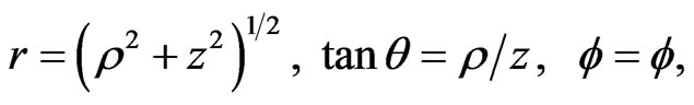 ,
,
 and
and 
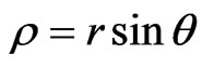
The contravariant and covariant forms  and
and  of the 4-velocity are
 (2)
(2)
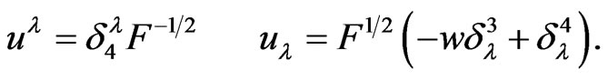
The electric 4-current , the electromagnetic 4-potential
  and the Faraday tensor
 , are
, are
 (3)
(3)
where  is the electric charge density. The EinsteinMaxwell field equations for charged dust are
 (4)
(4)
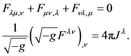 (5)
(5)
Here,  is the Einstein tensor
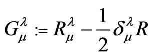 (6)
(6)
where  is the Ricci tensor of the spacetime defined by its fully covariant form as
 (7)
(7)
with  the Christoffel symbols of the second kind based on the metric of V in Equation (1),
 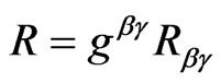 is the spacetime scalar curvature invariant and g is the determinant of
  The total stress-energy tensor
  is
is
 (8)
(8)
where
 (9)
(9)
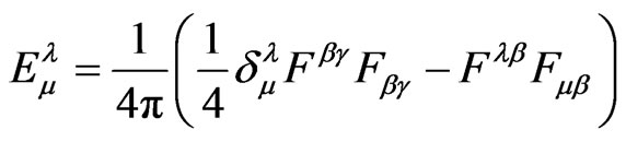 (10)
(10)
are, respectively, the matter and electromagnetic stressenergy tensors and  is the mass density.
Instead of expressing the electromagnetic field equations in 4-dimensional form as in Equations (5), we shall use the Maxwell form (Maxwell’s equations), because we can make direct comparisons with the results from classical electromagnetic theory. The electric and magnetic intensities and corresponding inductions in 3-vector form, are [4,5]
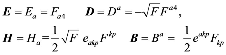 (11)
(11)
where ,
,  are the completely antisymmetric permutation tensors,
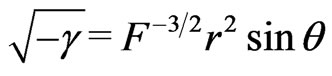
 ,
,  being the determinant of the spatial metric tensor
  which is given by
 with
with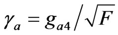 , and
, and  is the Levi-Civita symbol. It is easy to show that
 .
.
The transformed equations (2.14) and (2.13) of [2] may be written as
 (12)
(12)
 (13)
(13)
where the operators  and
and  are defined by
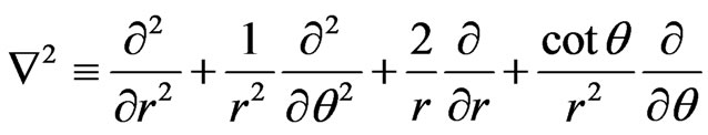 (14)
(14)
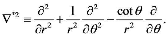 (15)
(15)
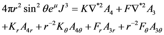
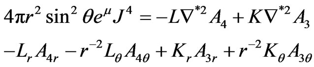
Equations (12) and (13) are the detailed form of the source-containing Maxwell equations given in the second of (5).
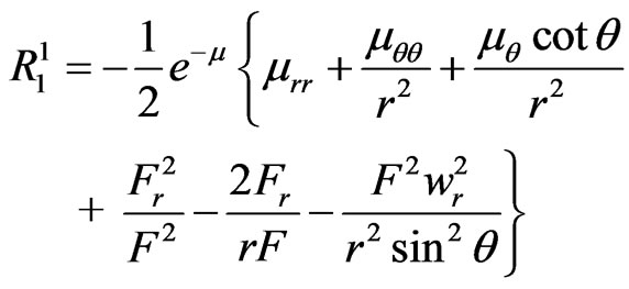
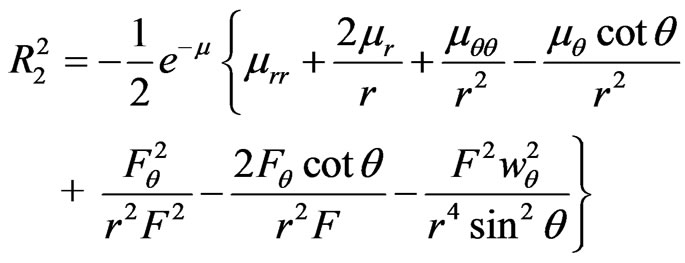
The non-zero components of the Ricci tensor obtained from the transformed Equations (2.16)-(2.21) of [2] are:
 (16)
(16)
 (17)
(17)
 (18)
(18)
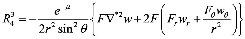 (19)
(19)
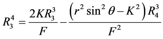 (20)
(20)
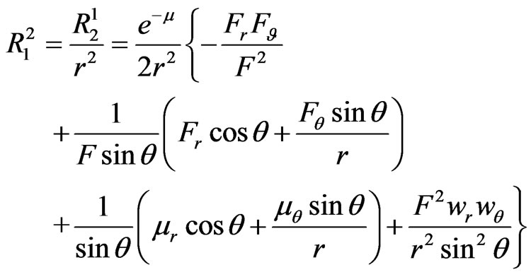 (21)
(21)
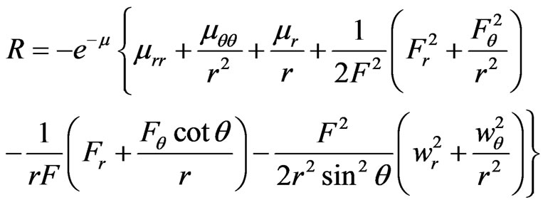 (22)
(22)
The entire Riemannian spacetime V, will be separated into the following 4-dimensional manifolds: the hypersurface  with equation
  separates V into the interior
  and exterior
 spacetimes. We shall use the + and – signs to denote quantities in
  and
and  whenever it is necessary to do so. Quantities without the + or – indicators, may be associated either with
  or with
 .
.
3. The Exterior Solution
In accordance with the formalism in [2], we first form the complex function
 (23)
(23)
where  and
and  are harmonic functions. With a star denoting complex conjugation, the metric functions
  and
and  are then given by
 . (24)
If we denote the real and imaginary parts of  by
by  and
and , then
 (25)
(25)
We now choose the functions  and
and  as follows:
 (26)
(26)
 (27)
(27)
where  and
and  are constants whose significance will emerge later. From now on we shall omit writing the argument
  of the Legendre polynomials and we shall write, for example,
  instead of
 . We note the significant fact that at
 ,
,  this enables us to set
  at
at 
 as in (27).
The function and the electromagnetic 4- potential
  in the exterior are obtained from
 (28)
(28)
 (29)
(29)
 (30)
(30)
 (31)
(31)
where an arbitrary constant in  was set equal to
  in order to satisfy the continuity condition of
  Note that the full expression for
  in the first of (28) is
 , but by (26),
 .
.
From Equations (24) and (28)-(31), we obtain the following expressions for 


and :
:
 (32)
(32)
 (33)
(33)
 (34)
(34)
 (35)
(35)
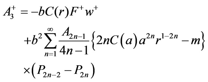
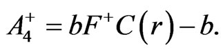
It is a little difficult to solve the two equations in (28) to find  in (33). It is even more difficult to solve the two Equations (29)-(30) to find
  in (34) and complete details of the calculation are not given. Whenever there are two signs in a term, the upper sign gives the expression in
  and the lower sign the expression in
  as in Equation (32).
The function B defined by
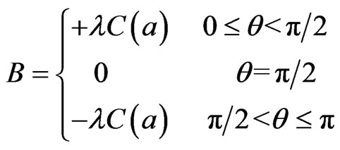 (36)
(36)
has Legendre polynomial expansion of the form
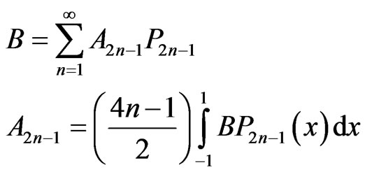 (37)
(37)
where  It therefore follows from (27), that
 . The function
 in (36) satisfies the conditions for such an expansion [6] and we have for the odd coefficients
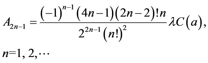 (38)
(38)
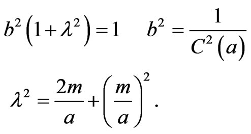
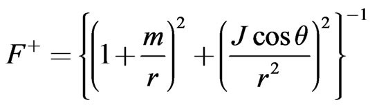
With  by Equations (24) and (26), the metric function F+ at
  becomes
 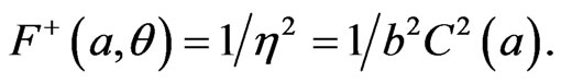 It will be shown in Section 4, that
  everywhere in the interior. In order to satisfy the junction condition at
  therefore, we must have
 . It is easily seen that, as
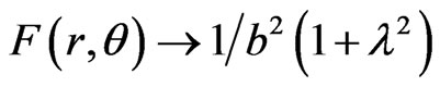 , which is a constant. If we take this to be equal to 1, we obtain
  and collecting these relationships together we have
 (39)
(39)
The third of Equation (39) is the result of substituting the second of these equations into the first, bearing in mind the second of Equation (26) for .
.
For the calculations that follow the functions and
and  defined by
 (40)
(40)
 (41)
(41)
will be required. We express  and
and  as
as
 (42)
(42)
The components of  are therefore calculated using the exterior functions (32)-(35) with Equations (16)-(22) and, whenever necessary, bearing in mind the first of Equation (39). The calculations give the following nonzero components:
 (43)
(43)
 (44)
(44)
 (45)
(45)
 (46)
(46)
 (47)
(47)
Here,  are the nonzero components of the electromagnetic energy tensor. The components of
  were obtained from (10) the third of (3) for
 , the exterior electromagnetic potentials in (34) and (35). Equation (22) gives
  in
in  and so by (6),
  whether
  is equal to
  or not. Another consequence of the result
 , is that the matter energy tensor
  will be null as should be the case in the electrovac
 .
.
The sourceless Maxwell equations in the first of (5) give  and
and . By the third of (3) and with
  and
and  given by (34) and (35), these become
 ,
,  which are trivially satisfied. The source-containing Maxwell Equations (12) and (13) with
  and
and  given by Equations (34) and (35) will give
  and
and  and so the 4-current is null in the electrovac
 .
.
4. The Interior Solution
In accordance with the results of [2], the functions  and
and  are constant which we shall take as
 (48)
(48)
The functions  and
and  satisfy an equation of the form
  with
with  given by (15). This implies that
  for example, is obtained from
 (49)
(49)
where  is a harmonic function, which therefore satisfies Laplace’s equation
  with
with  given by (14).
We choose  as
as
 (50)
(50)
where the constants  are determined from the junction condition
 . We use Equation (49) for
  with
with  given by (50) to find
 .
.
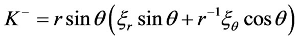
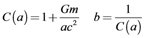
We can further show that

and with this, the above expression for  becomes

Finally, after a little manipulation, the above expression for  becomes
 (51)
(51)
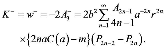
The junction condition for the continuity of K implies that on 
 . Using the expression (33) for w+ and bearing in mind that
  we have
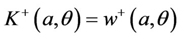 . It therefore follows from (33) and (51), that the constants
  are given by

This implies that , but also
  and
and  are given by
 (52)
(52)
The functions Z and U defined by
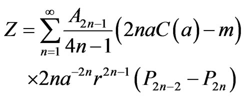 (53)
(53)
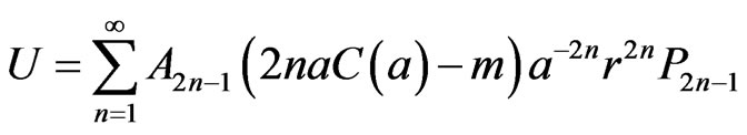 (54)
(54)
will be required to simplify the components of the Einstein tensor.
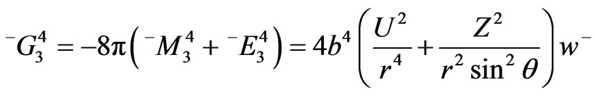
The components of  are calculated using the interior functions (48) and (52) with Equations (16)-(22) and, whenever necessary, bearing in mind the first of Equation (39). The calculations give the following nonzero components:
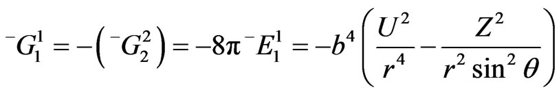 (55)
(55)
 (56)
(56)
 (57)
(57)
 (58)
(58)
 (59)
(59)
Here,  and
and  are the nonzero components of the electromagnetic and mass energy tensors respectively. The components of
  were obtained from (10) the third of (3) for
 , the interior functions in (48) and (52). The components of
  were obtained from Equations (3) and (9) together with the interior functions (48) and (52). Equations (55)-(59) state that Einstein’s Field Equations are satisfied in
 . The sourceless Maxwell equations in the first of (5) give
 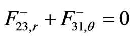 . By the third of (3) and with
  given in Equation (52), this becomes
 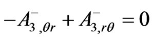 which is trivially satisfied. The source-containing Maxwell Equations (12) and (13) with
  and
and  as in (48) and (52) respectively, will give
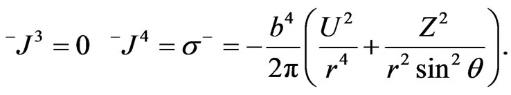 (60)
(60)
It is easily seen that
 .
.
It follows from this and Equation (60) that 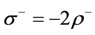 or, in dimensional units,
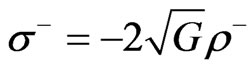 .
.
If N is any function in V, we write
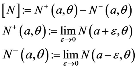 (61)
(61)
where the second and third of Equation (61), represent the values of  on the
  and
and  sides of
It follows from Equations (32)-(35), (48) and (52) that  and
and  The functions
  and
and  are therefore continuous across
  but one degree of smoothness is lost because the first order partial r-derivatives of these functions are discontinuous on
  It follows that the ordinary junction conditions requiring the continuity of the directional derivatives of these functions normal to
  cannot be applied. The discontinueties of these normal derivatives will generate a surface layer on
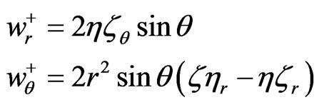
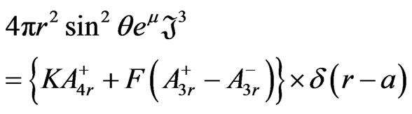
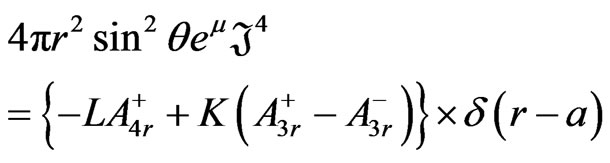
  with surface stress-energy tensor and surface 4-current and a more complicated set of junction conditions will apply. The Equations (12) and (13) for
  and
and  will give rise to expressions with factors of delta-functions and first order partial r-derivatives which are discontinuous on
  We shall denote these terms by Gothic symbols, and we find from (12) and (13) that these are
 (62)
(62)
 (63)
(63)
where  and
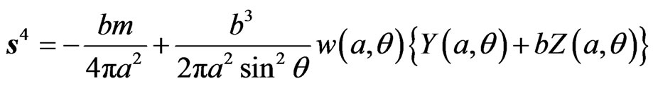
and  are given in (34), (35) and (52) respectively. To obtain the surface 4-current s and
 , we form the integrals of
  and
and  with respect to proper distance measured perpendicularly through
  from
from  to
to  and then find the limits as
  There are no sign indicators with the metric functions
  and
and  in (62) and (63) because their values in both,
  and
and , are required in these integrations, where the only nonzero contributions will arise from the delta-function parts
  and
and  of
of  and
and  in Equations (62) and (63). With
  the unit vector in the
  direction, this gives

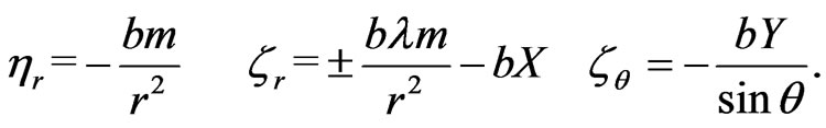
The electromagnetic junction conditions are

where  is the unit normal to the sphere and
  is the unit vector in the
  direction. In these equations, the contravariant component
  of
of  and the covariant component
  of
of  from the second and third of Equation (11) were used.
The Equations (16)-(22) for  and
and  will give rise to terms with factors of delta-functions and first order partial r-derivatives which are discontinuous on
 .
.
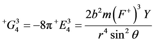
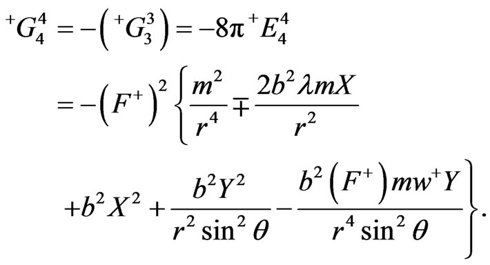
Denoting these terms by Gothic symbols, the Einstein tensor  and the associated matter stress-energy tensor
  are connected through the field equations, and so on
  we have
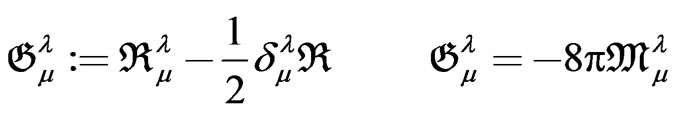 (64)
(64)
Bearing in mind that  and that in
 we display below the components
  and
and  as examples:
 .
.
The surface stress-energy tensor  is expressed in terms of the limits as
  of the integrals of
  with respect to r from
  to
to  and with
  given in Equations (64). The junction conditions on
  are [2,7]
 (65)
(65)
Here,  is the extrinsic curvature tensor of
  defined by
 , where the covariant differentiation is connected with the metric of
  Since
Since  on
on  this gives
 .
.
The hypersurface scalar curvature invariant of  is
is  where the Ricci tensor
  is given by
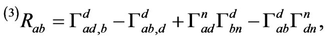
 being the Christoffel symbols of the second kind based on the metric of
 . With these, all the elements in the junction conditions (65) may be calculated and these conditions may be shown to be valid.
5. Mass, Charge, Angular Momentum and the Magnetic Dipole Moment
The mass, charge and angular momentum are defined by their imprints on the spacetime geometry far from the source. To obtain the gravitational mass and electric charge therefore, we expand the exterior metric function  up to the term
  Bearing in mind the first of (39), we then obtain from (32)
 (66)
(66)
We may transform  in (66) to the
  of the Reissner-Nordstrom solution, by the transformation
 giving
 with
with  [8], or in physical units,
 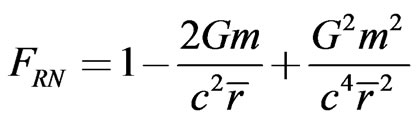 with
with
 . This expression therefore implies that the gravitational mass is
  and the electric charge is
  and these are connected by [8]
 (67)
(67)
If we now expand  to
to  we have
 (68)
(68)
where  is obtained from (38) by setting
  which will then give, bearing in mind (39)
 (69)
(69)
If  is the total angular momentum, we have [9]
 (70)
(70)
From (68) and (70), we then obtain  and on using (69), this gives
 (71)
(71)
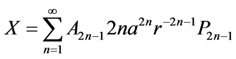
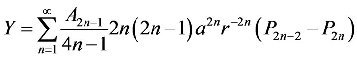
The dipole field is the part of the magnetic field  whose physical components
  and
and  contain the factors
  and
and  respectively. Since only the
  power is required, we only need the
  mode of the third of the expressions in (11) for
 . We find that these components are
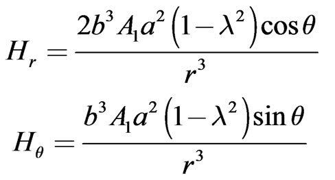 . (72)
With these, the magnetic dipole moment is therefore, 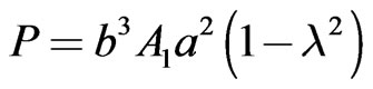 and on using (69), this gives
 (73)
(73)
From (71) and (73), we deduce that the gyromagnetic ratio is
 (74)
(74)
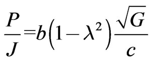
In physical units Equations (71), (73), (74) and the third of (39), become
 (75)
(75)
 (76)
(76)
 (77)
(77)
 (78)
(78)
It may be shown that the units of  and
and  are
are 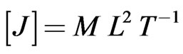 and
and 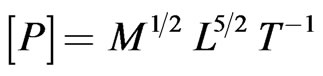 respectively, which are the units of angular momentum and magnetic dipole moment. We also find from the second of (26) and the second of (39) that
 (79)
(79)
We stress the fact that all the above formulae are for an electrically charged sphere whose mass m and charge q are related by Equation (67). We note from (75) and (76) that the angular momentum J and dipole moment P depend on  but also in a somewhat more subtle way, on the mass to radius ratio through the quantities
  and
and . The analytical Formula (77) may be applied to a number of different objects. We note that there exists a formula for the gyromagnetic ratio of stars known as Blackett’s empirical Formulas [10-12], which reads
 (80)
(80)
where  is a constant of the order of unity so that (80) becomes
 (81)
(81)
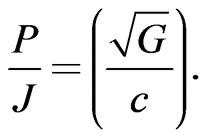
Blackett suggested that an explanation of this relation “must be sought in a new fundamental property of matter not contained within the structure of present day physical theory.” We note in this connection that the factor , occurs in both our analytical Formula (77) and in Blackett’s empirical Formula (80). The explanation for the presence of this factor in the analytical Formula (77) however is implicit in its derivation. Furthermore, the coefficient of
  in this formula is
 , and in Blackett’s Formula (80), it is a constant equal to 1, or approximately equal to 1. The quantity
  with
with  and
and  given by (78) and (79) respectively, is expected to vary from star to star, but
  in Blackett’s Formula (80) is a constant equal to 1 for all stars, an assertion that seems improbable. In the context of our solution, it is difficult to see why different objects which can be as diverse as the Earth and the Sun, will conform to such a requirement as implied by Blackett’s empirical Formula (81). Although the “new physics” idea was subsequently abandoned, it is nevertheless of interest to investigate further under what circumstances, if any, our exact analytical Formula (77) reduces to Blackett’s empirical Formula (81).
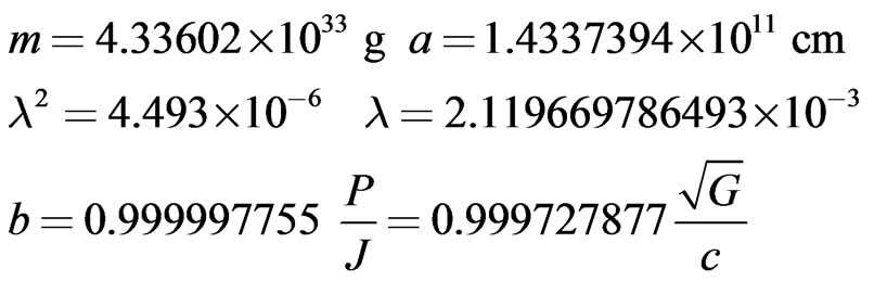
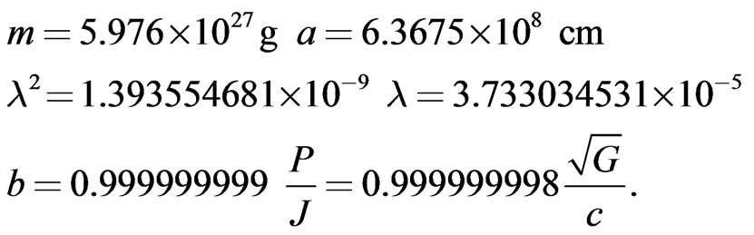
In order to gain an insight into the relation between the analytical Formula (77) and Blackett’s empirical Formula (81), we shall consider three cases with different numerical values for the radius  and gravitational mass
  of the sphere. We shall then proceed to calculate the corresponding quantities in
 ,
,  ,
,  and
and  in (78), (79) and (77):
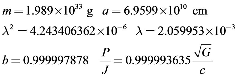 (82)
(82)
 (83)
(83)
 (84)
(84)
The above masses and radii were deliberately chosen to be numerically equal to those of the Sun, 78 Virginis and the Earth. These correspond to the three astronomical objects that are quoted in the literature by later authors in connection with Blackett’s empirical Formula (80) [10]. It is seen from the numerical results in (82)-(84), that in the case of our electrically charged spheres, the coefficient of  is very nearly equal to
 in every case. We must conclude that in situations where the ratio
  is such that
  is approximately equal to 1, our analytical Formula (77) will give Blackett’s empirical Formula (81). These reductions however, are only possible in the cases where,
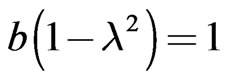 . Thus, if we consider a typical neutron star as a fourth case we have
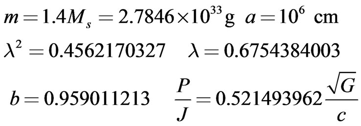 (85)
(85)
where  is the mass of the Sun.
It is seen that  and this is because
 . In the context of our equations, we found the precise condition under which our analytical Formula (77) will give Blackett’s empirical Formula (81). Again, in the context of our equations, this provides a full explanation why Blackett’s formula is sometimes valid and why this occurs only for a range of objects. Our formula for the gyromagnetic ratio
  is not empirical, but an exact analytical formula which is a consequence of the equations derived from the exact global solution of the Einstein-Maxwell field equations found here. It does not require any new fundamental properties of matter or any new physics and it is valid for all values of the ratio
 .
.
We note that Wilson [12,13] observed that in the case of the Earth and the Sun, the Formula (80) can be accounted for, if we assume that a rotating mass  has the same effect as a rotating electrical charge
  where
where  and
and  are connected by Equation (67). It is a little puzzling that our electrically charged spheres charged as they are in accordance with Equation (67), seem to echo the above observation by Wilson. In our case however,
  and
and  are connected by Equation (67) in reality. The quantity of charge required is quite small. As noted by Bonnor [8], if the mass
  and charge
  are related by Equation (67), then if in a sphere of neutral hydrogen one atom in 1018 had lost its electron, this would be sufficient.
6. Discussion and Conclusions
Exact exterior and interior solutions of the EinsteinMaxwell field equations for rigidly rotating pressure-free matter were obtained. The exterior and interior spacetimes are separated by a boundary which is a surface layer with surface stress-energy tensor and surface electric 4-current.
Perhaps one of the most important aspects of this work is that the source of spacetime, is rotating charged matter bounded by a closed surface. As far as we know, a global solution with a volume distribution of finite bounded rotating matter as a source of the spacetime, does not exist in the literature, although flat disk solutions do indeed exist [1]. Another important outcome of this work is the derivation of analytical formulae for the angular momentum, dipole moment and gyromagnetic ratio of a rotating sphere based on general relativistic equations.
The mass, charge, angular momentum and the magnetic dipole moment were determined in Section 5. In particular, we derived the analytical Formula (77) for the gyromagnetic ratio and discussed special cases to establish the facts regarding the connection between the analytical Formula (77) and Blackett’s empirical for Formula (80) the conditions under which the analytical Formula (77) reduces to Blackett’s empirical formula, were obtained. No new properties of matter and no new physics was required. Perhaps the analytical Formula (77) is valid for all rotating objects and in particular for stars, but we have no data to demonstrate this, except for the cases of the Sun, 78 Virginis and the Earth.
All the physical quantities of interest in the interior and exterior were calculated as well as those associated with the spherical surface layer. In this problem, the ordinary gravitational junction conditions are inappropriate. In fact there are two sets of junction conditions, the electromagnetic and the gravitational ones. The former were expressed in the familiar form of classical electromagnetic theory. The gravitational junction conditions in this problem are more complicated than the usual ones, because of the surface layer. These were clearly stated, although no detailed formulae were displayed.
This solution permits a reversal of the signs of  and
and  in (34) and (35) [14], which will cause a reversal of the signs of
  and
and  in (52) and (48). If we replace the harmonic functions
  and
and  in (26) and (27) by

then, instead of the metric functions in (32) and (33), we shall have

with appropriate modifications to the remaining functions in (32)-(34). Our exterior solution, given by these equations, reduces to the solution obtained by Perjes [14].
To find the limit of the exterior solution (32)-(35) when the angular momentum  is reduced to zero, we replace the harmonic function
  in (27) by zero, choose
  and base the solution on the single harmonic function
  in (26). This leads to

which is the Papapetrou solution [15] for which Bonnor has found a matching interior solution [8].
Referring to the surface layer that occurs in our solution, we note the result obtained by Ruffini and Treves in a non-relativistic treatment, in which they had shown that a magnetized rotating object has surface charge and current densities; it is also endowed with a net electric charge [16]. This agrees with our results and in particular, it confirms the existence of a surface layer with 4-current and stress-energy tensor on the boundary 
The mass, charge, angular momentum and the magnetic dipole moment were determined in Section 5. In particular, we derived the analytical Formula (77) for the gyromagnetic ratio and discussed special cases to establish the facts regarding the connection between the analytical Formula (77) and Blackett’s empirical Formula (80). The conditions under which the analytical Formula (77) reduces to Blackett’s empirical formula, were obtained. No new properties of matter and no new physics were required. Perhaps the analytical Formula (77), is valid for all rotating objects and in particular for stars, but we have no data to demonstrate this, except for the cases of the Sun, 78 Virginis and the Earth.
REFERENCES
- M. A. H. MacCallum, M. Mars and P. Vera, “Stationary Axisymmetric Exteriors for Perturbations of Isolated Bodies in General Relativity, to Second Order,” Physical Review D, Vol. 75, 2007, Article ID: 024017.
- A. Georgiou, “Rotating Einstein-Maxwell Fields: Smoothly Matched Exterior and Interior Spacetimes with Charged Dust and Surface Layers,” Classical and Quantum Gravity, Vol. 11, No. 1, 1994, pp. 167-186. doi:10.1088/0264-9381/11/1/018
- W. Bonnor, “Rotating Charged Dust in General Relativity,” Journal of Physics A: Mathematical and General, Vol. 13, 1980, pp. 3465-3477.
- A. Georgiou, “Comments on Maxwell’s Equations,” International Journal of Mathematical Education in Science and Technology, Vol. 13, No. 1, 1982, pp. 43-47. doi:10.180/0020739820130106
- C. Moller, “The Theory of Relativity,” 2nd Edition, Oxford University Press, Oxford, 1972.
- E. T. Whittaker and G. N. Watson, “A Course of Modern Analysis,” 4th Edition, Cambridge University Press, Cambridge, 1950.
- W. Israel, “Singular Hypersurfaces and Thin Shells in General Relativity,” Nuovo Cimento B, Vol. 48, No. 2, 1966, p. 463. doi:10.1007/BF02712210
- W. Bonnor, “The Equilibrium of a Charged Sphere,” Monthly Notices of the Royal Astronomical Society, Vol. 129, 1965, p. 433. http://adsabs.harvard.edu/abs/1965MNRAS.129.443B
- J. N. Islam, “Rotating Fields in General Relativity,” Cambridge University Press, Cambridge, 1985. doi:10.1017/CB09780511735738
- P. M. S. Blackett, “The Magnetic Field of Massive Rotating Bodies,” Nature, Vol. 159, No. 4046, 1947, pp. 658- 666.
- D. V. Ahluwalia and T. Y. Wu, “On the Magnetic Field of Cosmological Bodies,” Lettere Al Nuovo Cimento, Vol. 23, No. 11, 1978, pp. 406-408. doi:10.1007/BF02786999
- J. A. Nieto, “Gravitational Magnetism and General Relativity,” Revista Mexicana de Fisica, Vol. 34, No. 4, 1988, pp. 571-576.
- H. A. Wilson, “An Experiment on the Origin of the Earth’s Magnetic Field,” Proceedings of the Royal Society, Vol. 104A, 1923, p. 451. http://www.jstor.org/stable/94216
- Z. Perjes, “Solutions of the Coupled Electromagnetic Equations Representing the Fields of Spinning Sources,” Physical Review Letters, Vol. 27, 1971, p. 1668.
- A. Papapetrou, “A Static Solution of the Equations of the Gravitational Field for an Arbitrary Charge-Distribution,” Proceedings of the Royal Irish Academy, Vol. 51, 1945- 1948, p. 191.
- R. Ruffini and A. Treves, “On a Magnetized Rotating Sphere,” Astrophysical Journal Letters, Vol. 13, 1973, p. 109.