ABSTRACT

In this paper, a reliable computational tool will be developed for the determination of the parameters of the stellar density function in a region of the sky with complete error controlled estimates. Of these error estimates are, the variance of the fit, the variance of the least squares solutions vector, the average square distance between the exact and the least-squares solutions, finally the variance of the density stellar function due to the variance of the least squares solutions vector. Moreover, all these estimates are given in closed analytical forms.

Keywords:Astrostatistics, Stellar Density Function, Computational Astrophysics

1. Introduction

Modern observational astronomy has been characterized by an enormous growth of data stimulated by the advent of new technologies in telescopes, detectors and computations. The new astronomical data give rise to innumerable statistical problems [1] . Moreover, empirical astrophysics researches have seen a paradigm shift in recent years in that it routinely involves data mining of large multi wavelength data sets, requiring complex automated processes that must invoke a very diverse set of statistical techniques (e.g. [2] [3] ).

On the other hand, one of the most crucial pieces of information needed in astronomy is the stellar density function in a region of the sky, due to the wealth of information on galactic structure gained directly from a study of the variations in the stellar density (e.g. [4] -[6] ).

Although the least-squares method is the most powerful technique that has been devised for the problems of astrostatistics in general [7] , it is at the same time exceedingly critical. This is because the least-squares method suffers from the deficiency that, its estimation procedure does not have detecting and controlling techniques for the sensitivity of the solution to the optimization criterion of the variance is minimum. As a result, there may exist a situation in which there are many significantly different solutions that reduce the variance to an acceptable small value.

At this stage we should point out that 1) the accuracy of the estimators and the accuracy of the fitted curve are two distinct problems; and 2) an accurate estimator will always produce small variance, but small variance does not guarantee an accurate estimator. This could be seen from Equation (2) by noting that the lower bounds for the average square distance between the exact and the least-squares values is which may be large even if is very small, depending on the magnitude of the minimum eigenvalue, , of the coefficient matrix of the least-squares normal equations. Unless detecting and controlling this situation, it is not possible to make a well-defined decision about the results obtained from the applications of the least squares method.

The importance of the stellar density function as mentioned very briefly as in the above and the existing practical difficulties due to the deficiency of the error estimation and controlling had motivated our work: to develop a reliable computational tool for the determination of the parameters of the stellar density with complete error estimates. Of these error estimates are, the variance of the fit, the variance of the least squares solutions vector, the average square distance between the exact and the least-squares solutions, finally the variance of the density stellar function due to the variance of the least squares solutions vector.

By this we aim at giving an idea on what may called an “accepted solution set” for the parameters of the stellar density functions and the associated variances by the selected tolerances for the error estimates.

Before starting the analysis, it is profitable, to give brief notes on the structure of the paper as follows.

1-Using Fourier transform to obtain analytical solution of the density function;

2-Using the least squares method to find second order polynomial for each of the apparent and absolute magnitudes distributions;

3-Using steps 1 & 2, we established analytical expressions of the density function with coefficients directly obtained from observations.

2. Linear Least Squares Fit

Let be represented by the general linear expression of the form:

where are linear independent functions of. Let be the vector of the exact values of the coefficients and the least squares estimators of obtained from the solution of the normal equations of the form. The coefficients matrix is symmetric positive definite, that is, all its eigenvalues are positive. Let E(z) denotes the expectation of z and the variance of the fit, defined as:

where

is the number of observations, is the vector with elements and has elements. The transpose of a vector or a matrix is indicated by the superscript “”.

According to the least squares criterion, it could be shown that [8]

1-The estimators obtained by the least squares method gives the minimum of.

2-The estimators of the coefficients, obtained by the least squares method, are unbiased; i.e..

3-The variance-covariance matrix of the unbiased estimators is given by:

(1)

where is the inverse of the matrix.

4-The average squared distance between and is:

. (2)

Also it should be noted that, if the precision is measured by probable error, then:

.

Finally, if is a linear function of the independent variables given by

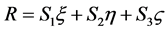, (3.1)

then [9]

, (3.2)

where is the variance of and are the variances of the independent variables

3. Basic Equations

3.1. The Integral Equation of the Problem

The absolute magnitude, M of a star is given in terms of the apparent magnitude and parallax (in second of arc) by

where M is thus defined in terms of the standard distance of 10 parsecs. We write, for convenience,

so that is defined in terms of the standard distance of 1 parsec, and

.

In the above formulae the base of the logarithm is 10.

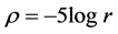
We shall refer to in this connection as the modified absolute magnitude. Also, with r measured in parsecs, we have and

.

Let be the frequency function of and denote the total number of stars with apparent magnitude between and in small region of the sky subtends a solid angle in the distance interval  and where the density function is, then (Trumple & Weaver1953)

.

Let

then

Let

then

.

Consequently

Hence

or

(4)

where

, (5)

. (6)

Equation (4) is the basic integral equation to be solved for the density function as will be shown latter.

3.2. Maxwellian Distributions of the Magnitudes

Let the distributions of the apparent and absolute magnitudes are Maxwellian in form. We assume that

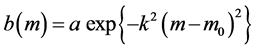, (7.1)

, (7.2)

. (7.3)

As regards Equation (7.1), this is the form found to satisfy the star counts for a given galactic latitude in the exhaustive investigation by many authors. The parameters, and are to be regarded as functions of galactic latitude and possibly also of galactic longitude.

Equation (7.2) must be regard as applicable only to a particular spectral type or subdivision of spectral type. In many studies of the distribution of absolute magnitudes, the separation of stars into the giant and dwarf classes is recognized, that in dealing with a given spectral type we represent the function as the sum of two Maxwellian expressions of the type (7.2). In the following analysis, we deal with a single Maxwellian function only.

The condition (7.3) implies that the dispersion about the mean is less for absolute magnitudes of a given spectral type than for the apparent magnitudes. This is in accordance with observations, for the giants or for the dwarfs.

4. The Normal Equations and the Associated Error Analysis

Taking the natural logarithm of Equations (7.1) and (7.2) we get,

, (8)

where

(9)

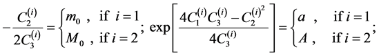(10)

and stands for if and for if

Since, are known from observations for all, then according to Section2,the normal equations associated with Equations (8) are:

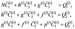(11)

where

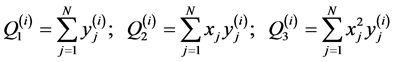(12)

(13)

In the following two sections, the solutions of the normal equations for together with the associated error analysis will be developed in closed analytical forms.

4.1. Solutions of the Normal Equations

The solutions of the normal Equations (11) for are given exactly as,

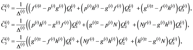(14)

where

. (15)

4.2. Error Analysis

According to Section 2, we deduce for, that:

1-The variance of the fit is:

(16)

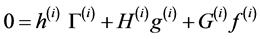
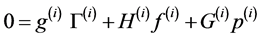
2-The variance of the solutions are:

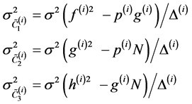, (17)

3-The average squared distance between the least square solutions and the exact solutions is

. (18)

5. Analytical Expression of the Density Function D(r)

Recalling the Fourier transform of the function as:

(19.1)

while its inverse is

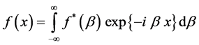. (19.2)

Multiply Equation (4) by and integrate between, then

, (20)

where

.

Let then,

also

,

.

Then Equation (20) reduces to

also

.

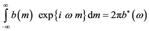
The inverse of Fourier transform of is:

then

, (21)

where and are the Fourier integrals of and respectively where

;

could written as

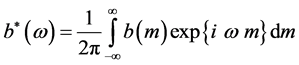. (22)

Using Equation (7.1) in Equation (22) the later becomes:

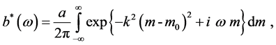
or, on setting,we get:

evaluating the integral on the right hand side we get

(23)

Similarly, as in deriving Equation (23) we can get for the expression:

(24)

Now, substituting Equations (23) and (24) into Equation (21) we get,

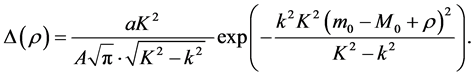
Using Equation (6) and remembering that we obtain for the density function the expression:

. (25)

6. Empirical Determination of the Density Function D(r) and Its Accepted Solution Set

In what follows empirical expression of the density function and its variance will be established in literal closed forms.

6.1. Empirical Expression

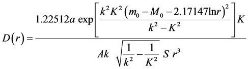
Substituting Equations (9) and (10) into Equation (25), we get for the density function the empirical expression

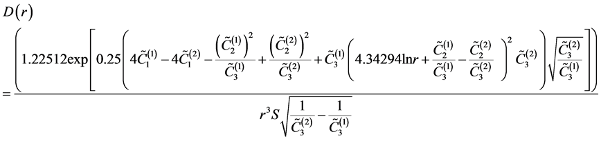(26)

where are the solutions of the normal equations (Equations (14))

6.2. The Variance

Since function of, then what is the variance due to the variances? The following analysis is devoted for the answer of this question.

Define

(27.1)

(27.2)

, (28.1)

, (28.2)

, (28.3)

therefore we have

, (29.1)

, (29.2)

, (29.3)

, (30.1)

, (30.2)

. (30.3)

From Equations (29) we get

, (31.1)

, (31.2)

. (31.3)

Multiply Equations (28.1) and (28.2) and then summing, we get

, (32.1)

similarly

, (32.2)

. (32.3)

Since

, (33)

then summing we have

, (34.1)

similarly

(34.2)

. (34.3)

Multiply Equation (33) by and summing we get

, (35.1)

similarly

, (35.1)

, (35.2)

, (35.3)

, (35.4)

. (35.5)

Since are the least squares solutions, then the corresponding residual, is given by:

, (36)

consequently,

. (37)

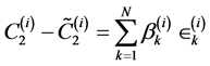
According to Section 2, we have

. (38)

where are the exact values of the unknowns and is the error associated with.

Multiply Equations (38) and (37) by, subtracting, then summing we get

, (39.1)

similarly

, (39.2)

, (39.3)

let us take the error, , of the density function in the sense

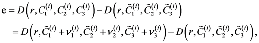
then assuming that the errors in Equations (39) are small, then we can write with sufficient accuracy by means of Taylor expansion as:

where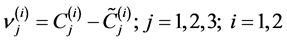,then using Equations(39) we get

(40)

where

.

Now, in Equation (40), e is linear function of the errors; hence, then according to Equation (3) we have

.

Using Equations (31), (32) and (17) we finally get

, (41)

where are given as

, (42.1)

, (42.1)

(42.3)

, (42.4)

(42.5)

(42.6)

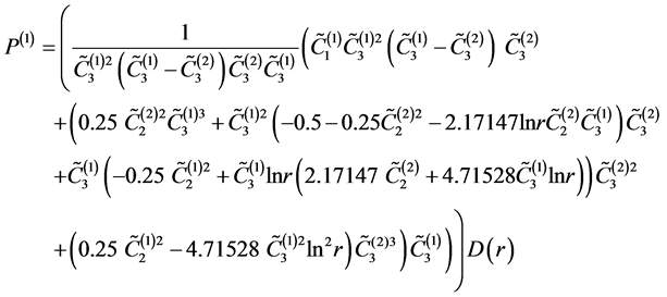
6.3. The Variances of k², K², m₀, M₀, a, A

Since each of the constants is a function of the least squares solutions, the by the same arguments as for Equations (42) we get

(17)

(43.1)

(43.2)

(43.3)

where

(44)

6.4. An Accepted Solution Set for D(r)

Due to the above mentioned practical difficulties encountered in most applications of the least squares method we should at this stage reformalize the concept of an “acceptably small” variance. We may define an acceptable solution set to the determination of as:

(45)

where Tol and small numbers. In writing Equation (45) we do not mean to establish this particular definition of an acceptable solution set, as it is only intended to give the users of the least squares method for some degree of concreteness to the general idea of an acceptable solution set.

5. Conclusion

In conclusion, a reliable computational tool was developed in the present paper for the determination of the parameters of the stellar density function in a region of the sky with complete error controlled estimates. Of these error estimates are, the variance of the fit, the variance of the least squares solutions vector, the average square distance between the exact and the least-squares solutions, finally the variance of the density stellar function due to the variance of the least squares solutions vector. Moreover, all these estimates are given in closed analytical forms.

References

- Feigelson, E.D and Babu, J.B (2012) Modern Statistical Methods for Astronomy with Applications. Cambridge University Press, Cambridge.
- Sharaf, M.A, Issa, I.A. and Saad, A.S. (2003) Method for the Determination of Cosmic Distances. New Astronomy, 8, 15-21. http://dx.doi.org/10.1016/S1384-1076(02)00198-7
- Sharaf, M.A. and Sendi A.M. (2010) Computational Developments for Distance Determination of Stellar Groups. Journal of Astrophysics and Astronomy, 31, 3-16. http://dx.doi.org/10.1007/s12036-010-0002-0
- Trumpler, R.J. and Weaver, H.F. (1953) Statistical Astronomy. Dover Publication, Inc., New York.
- Robinson, R.M. (1985) The Cosmological Distance Ladder. W.H. Freeman and Company, New York.
- Binney, J. and Merrifield, M. (1998) Galactic Astronomy. Princeton University Press, Princeton.
- Andreon, S. and Hurn, M. (2013) Measurement Errors and Scaling Relations in Astrophysics: A Review. Statistical Analysis and Data Mining: The ASA Data Science Journal, 6, 15-33.
- Kopal, Z. and Sharaf, M.A. (1980) Linear Analysis of the Light Curves of Eclipsing Variables. Astrophysics and Space Science, 70, 77-101. http://dx.doi.org/10.1007/BF00641665
- Bevington, P.R and Robinson, D.K. (1992) Data Reduction and Error Analysis for the Physical Sciences. McGraw-Hill, New York.