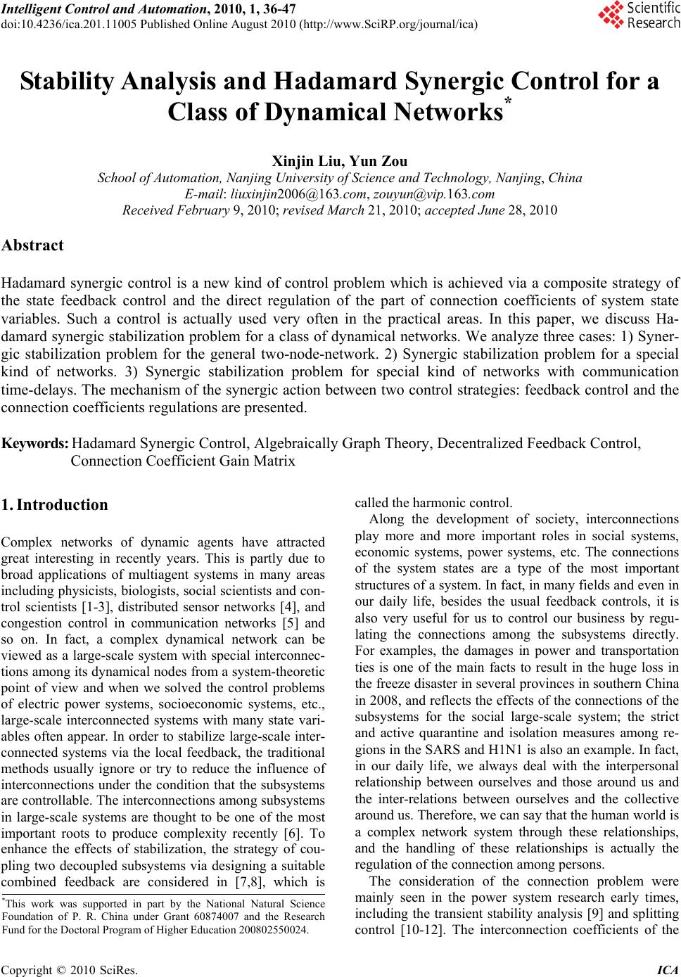Intelligent Control and Automation, 2010, 1, 36-47
doi:10.4236/ica.201.11005 Published Online August 2010 (http://www.SciRP.org/journal/ica)
Stability Analysis and Hadamard Synergic Control for a
Class of Dynamical Networks*
Xinjin Liu, Yun Zou
School of Automation, Nanjing University of Science and Technology, Nanjing, China
Received February 9, 2010; revised March 21, 2010; accepted June 28, 2010
Abstract
Hadamard synergic control is a new kind of control problem which is achieved via a composite strategy of
the state feedback control and the direct regulation of the part of connection coefficients of system state
variables. Such a control is actually used very often in the practical areas. In this paper, we discuss Ha-
damard synergic stabilization problem for a class of dynamical networks. We analyze three cases: 1) Syner-
gic stabilization problem for the general two-node-network. 2) Synergic stabilization problem for a special
kind of networks. 3) Synergic stabilization problem for special kind of networks with communication
time-delays. The mechanism of the synergic action between two control strategies: feedback control and the
connection coefficients regulations are presented.
Keywords: Hadamard Synergic Control, Algebraically Graph Theory, Decentralized Feedback Control,
Connection Coefficient Gain Matrix
1. Introduction
Complex networks of dynamic agents have attracted
great interesting in recently years. This is partly due to
broad applications of multiagent systems in many areas
including physicists, biologists, social scientists and con-
trol scientists [1-3], distributed sensor networks [4], and
congestion control in communication networks [5] and
so on. In fact, a complex dynamical network can be
viewed as a large-scale system with special interconnec-
tions among its dynamical nodes from a system-theoretic
point of view and when we solved the control problems
of electric power systems, socioeconomic systems, etc.,
large-scale interconnected systems with many state vari-
ables often appear. In order to stabilize large-scale inter-
connected systems via the local feedback, the traditional
methods usually ignore or try to reduce the influence of
interconnections under the condition that the subsystems
are controllable. The interconnections among subsystems
in large-scale systems are thought to be one of the most
important roots to produce complexity recently [6]. To
enhance the effects of stabilization, the strategy of cou-
pling two decoupled subsystems via designing a suitable
combined feedback are considered in [7,8], which is
called the harmonic control.
Along the development of society, interconnections
play more and more important roles in social systems,
economic systems, power systems, etc. The connections
of the system states are a type of the most important
structures of a system. In fact, in many fields and even in
our daily life, besides the usual feedback controls, it is
also very useful for us to control our business by regu-
lating the connections among the subsystems directly.
For examples, the damages in power and transportation
ties is one of the main facts to result in the huge loss in
the freeze disaster in several provinces in southern China
in 2008, and reflects the effects of the connections of the
subsystems for the social large-scale system; the strict
and active quarantine and isolation measures among re-
gions in the SARS and H1N1 is also an example. In fact,
in our daily life, we always deal with the interpersonal
relationship between ourselves and those around us and
the inter-relations between ourselves and the collective
around us. Therefore, we can say that the human world is
a complex network system through these relationships,
and the handling of these relationships is actually the
regulation of the connection among persons.
The consideration of the connection problem were
mainly seen in the power system research early times,
including the transient stability analysis [9] and splitting
control [10-12]. The interconnection coefficients of the
*This work was supported in part by the National Natural Science
Foundation of P. R. China under Grant 60874007 and the Research
Fund for the Doctoral Program of Higher Education 200802550024.

X. J. LIU ET AL.
37
state variables of the subsystems are considered as the
control variables that are regulated directly in the split-
ting control for power system. Furthermore, the isolation
treatment strategy is further discussed in the emergency
control [13-15]. The studies give a theoretical interpreta-
tion for the practical experiences that the early quaran-
tine and isolation strategies are critically important to
control the outbreaks of epidemics. Finally, a new kind
of concept called Hadamard synergic control is intro-
duced based on the Hadamard matrix product [16]. It is
achieved via a composite strategy of the state feedback
control and the direct regulation of the part of connection
coefficients of system state variables. Such a control im-
proves the limitations of the traditional feedback control
[17-19] and may be of some potential applications in the
emergency treatment such as isolation and obstruction
control. For clear, we give this model again here.
Consider the following linear time-invariant system:
 
x
tAxtBut
 (1)
Here,

,,,1,2,,
Tm
iji i
nn
A
aBbbRin



 
Obviously, the element ij a is the interconnection co-
efficient between the i-th state and the j-th state, for con-
venience, we call the system matrix A as system inter-
connection matrix. In many practical cases, such as the
switches and circuit breakers in the power systems, fire-
wall in the Internet etc., the system interconnection ma-
trix A can be directly regulated, of course, can be
pre-designed in some extent. Thus, the system intercon-
nection matrix A can be divided into two parts: 12
A
A

.
1
A
is the fixed part of A which is not able to be regu-
lated directly and 2
A
is the flexible part of A which can
be regulated directly in some extent. By using the Ha-
damard matrix product, this direct regulation of the in-
terconnection matrix A can be written as follows:
12K
A
AAK (2)
Here, for convenience, we call []
ijn n
Kk

 as the
connection coefficient gain matrix. It may be need to
satisfy some constraints such as 01
ij
k etc. Of
course, the control strategy above is different from the
feedback control. 2
A
K is the Hadamard matrix prod-
uct defined as [20]:
22
,
ij ijij
nn nn
AK akAa

 

 


Then, the general feedback control problem formula-
tion can be extended as follows: find direct connection
coefficient gain matrix K and feedback gain matrix
F
such that the generalized closed loop system

12
x
AAKBFx 
 (3)
is stable, robust stable, or some other specific perform-
ances. For convenience, we call this kind of control
strategy as Hadamard synergic control.
In order to illustrate the idea of isolation and obstruc-
tion of the connections among subsystems, we give the
following examples [21].
Example 1. Replacing the scalars ,, ,
ij ij ij
abfk by
matrices , ,,
ijijij ij
A
BFkE with appropriate dimensions
and the self-loops are not allowed, the general Hadamard
synergic control model (3) can be rewritten as:
111 1121221111 1
222 2212112222 2
11111 1
nnn
nnn
nnn nnnnnnnnnn n
xAxkAx kAxBu
xAxkAxkAxBu
x
AxkAxkAxBu

  
 
 




Where ,1,2,,
i
n
i
x
Ri n is the local state of the i-th
subsystem. ij kare the control variables. System model
above can be rewritten as:


12
x
AAKxBu 
 (4)
Here,
12 1
11
21 2
12
12
12 1211
11
21 2122
112 2
0
0
,
0
0
0
,
0
[1] ij
n
n
nn
nn
nn
nn
nn
nnn n
ijn n
AA
AAA
AA
AAA
kE kE
BkE kE
BK
BkEk E
E







































In power systems, the model (4) can be used to describe
the frequency control in multi-areas loads with the bal-
ance of active powers among the networks of different
areas.
Example 2. Consider the network model researched in
[1,3], in fact, the system interconnection matrix
A
is
divided into two parts. By the Kronecker product, this
network model can be written as [22]:

 
1nOC n
x
IACAxIBu 
 (5)
Where

12 12
,,, ,,,,
TT
TT TTT T
nn
x
xxxu uuu,nn CR


is called as the outer coupling matrix, C
A
is the inner
coupling matrix describing the interconnections.
Obviously, the network model (5) is a special case of
the model (4). From the definition of the matrix Kronecker
product we know, the connection matrix of the system
has very symmetrically consistency structure if we de-
scribe the system by using the corresponding Hadamard
product, this is: any two subsystems have the same basic

X. J. LIU ET AL.
38
connection structure except the coupling coefficient, i.e .
11 22
1, 2,,
1
O
ij
C
nn
A
ij n
A
A
ijn
BB B







Network model (5) has very specific project back-
ground such as in the consensus and formation control
problem. This also illustrates the rationality and general-
ity of the abstract model (4).
Example 3. The host population consists of six sub
populations: namely susceptible individuals 1()
x
t, as-
ymptomatic individuals 2()
x
t, quarantined individuals
3()
x
t, symptomatic individuals 4()
x
t, isolated indi-
viduals 5()
x
t, recovered individuals 6()
x
t. The total
population size is
6
1
()
i
i
Nxt

. The detailed descrip-
tions of other parameters see [23]. The SARS transmis-
sion model with quarantine and isolation controls u and v
is given by the following nonlinear system of differential
equations:




4235
11
4235
212
3223
412 114 4
542322 5
61425 6
EQJ
EQJ
xxxx
xx
N
xxxx
x
pkux
N
xux kx
xkx dxvx
xvxkxdx
xxxx
 
 



 

 

 

 
 






Obviously, the model above is a typical interconnec-
tion-regulation control of a nonlinear system with the
control variables u and v (see Figure 1).
Hadamard product is a classical matrix product. It has
many applications in some areas especially in mathe-
matics and physics. It also has some applications in sig-
nal processing [24]. In the existing literatures, almost all
the results about the eigenvalue estimations on Ha-
damard products were obtained under the presupposition
that the involved matrices are special ones such as
M-matrices, Hermitian (or the form of *
A
A), diagonal
matrices, etc. See [25-29] and the other corresponding
references. Also, the discussions on the mixture products
like ()
A
BC are scarcely reported. Hence, the basic
properties and expressions on Hadamard product still
remain to be extensively studied.
Although almost all the existing control theory and
applications are implemented by feedback controls, the
feedback is, in a general sense, only one of the specific
measures to implement the regulations of the connections
of system states.
)(
1
tx

1
x



tx
2
p
2
x



tx
4
21
xk
4
x

41
xd

 tx
6
41
x


 tx
3
2
ux
3
x

32
xk
 tx
5
5
x

52
xd
4
vx
52
x

6
x

Figure 1. A schematic representation of the populations
flow.
Let the feedback law be,mn
j
uFxF fR



 ,
,1,2,,
m
j
f
Rj n. Then the system matrix of the
closed loop is of the form: T
ijijnn
Aabf




. The ac-
tual functions of the feedback are the compensations of
ij
a, i.e., regulating the interconnection coefficients from
ij
a to T
ijij
abf via the input information channel.
Hence, in an open-loop viewpoint, the feedback control
is just a special indirect regulation of interconnections of
system states.
The observation above show that the feedback control
strategy is only one of the specific measures to imple-
ment the regulations of the connections of system states
via the input information channel, rather than the direct
physical regulation of the system interconnection matrix
A.
In this paper, we mainly discuss the Hadamard synergic
stabilization problem for the general two-node-network
(4), and then Hadamard synergic stabilization problem
for the special model (5) is studied. Matrix algebra and
algebraic graph theory are proved useful tools in model-
ing the communication network and relating its topology
to the discussion of the network stability.
The rest of this paper is organized as follows. System
models and problem formulation discussed in this paper
are given in Section 2. Hadamard synergic stabilization
problem for the general two-node-network (4) is studied
in Section 3. In Section 4, Hadamard synergic stabiliza-
tion problem for the special network model (5) is dis-
cussed. Furthermore, networks with communication
time-delays are investigated. The last section concludes
the paper.
2. System Models and Problem Formulation
In this section, we give the system models and problem
formulation discussed in this paper.
Because of the existence of the Hadamard product,

X. J. LIU ET AL.
39
this makes that the stability analysis of the general net-
work model (4) become difficult. Therefore, we mainly
consider the Hadamard synergic control problem for the
special model (5). Furthermore, Hadamard synergic con-
trol for the two-node-network model of the general net-
work system (4) is investigated simply. For convenience,
the network model (5) can be rewritten as:

1nOC n
x
IAKAxIBu 
 (6)
ij nn
Kk

  is the connection coefficient gain matrix.
In the general case, the control variables ij
k often
need to satisfy some constraints. There exist the follow-
ing cases being researched.
Case 1: ij k is discrete. For example 0,1
ij
k. When
0
ij
k, it means that we cut off the connections from the
j-th subsystem to the i-th subsystem; When 1
ij
k

, it
means that we keep the corresponding connections. In
this case, the control is called the isolation treatment
strategy. In fact, this kind of control strategy has been
researched in many literatures [15] especially in the
power electrical engineering [10-12].
Case 2: ij k is continuous. It often needs to meet
some constraints. For example, 01
ij
k in the epi-
demic control [13,14,25];
n
ii ij
ji
kk


 in the consensus
or formation control problem [30,31], etc.
Although the control variables ij
k often need to sat-
isfy some constraints, as the stability research in the
classical feedback control of the system (1) required to
unconstrained control ()ut we also suppose that the
connection coefficient ij kR in this paper.
We present the formulations of the Hadamard synergic
stabilization problems as follows:
Hadamard synergic stabilization problem (HSSP)
[21]: Given system (1), and let 12
A
AA . Find con-
nection coefficient gain matrix nn
K
R  and feedback
control uFx such that the corresponding Hadamard
synergic closed loop (3) is stable, i.e.

12
A
AKBFC 


Where (.)

represents the set of eigenvalues of the
corresponding matrix, C means the left-half complex
plane. For convenience, we call the matrix pair ),( FK
as the synergic control matrix pair.
Remark 1. Obviously, the HSSP is equivalent to the
problem that is to find connection coefficient gain matrix
K such that 12 (,)
A
AKB is stabilizable. One of the
stronger conditions of it is to find a matrix K such that
12
(,)
A
AKB is completely controllable. Also, for
convenience, we call these two problems as Hadamard
synergic stabilization and Hadamard synergic Controlla-
bilization problems respectively.
In this paper, we mainly consider the Hadamard syn-
ergic stabilization problem for the two cases:
Case 1: The two-node-network model of the general
network system (4).
Case 2: The special network model (6).
3. Hadamard Synergic Stabilization for THE
General Two-Node-Network
In this section, we consider the Hadamard synergic Sta-
bilization problem for the general dynamical network
model (4). We mainly consider the two-node-network de-
scribed as:
111 11212211 1
22222121 1222
x
AxAx Bu
x
AxAxBu


 
 

 (7)
Then, the Hadamard synergic stabilization problem for
the network model (7) can be presented as: find connec-
tion coefficients 1221 ,R



and decentralized feed-
back control 1112 22 ,uFxu Fx

 such that the closed
loop matrix
111111212
21 212222 2
(2)
loop
ABFA
A
A
ABF











is stable.
When 12 0


or 210


, the stability of (2)
loop
A
is equal to the stability of the two subsystems, so we do
not consider this condition. In the following, we suppose
that 1221 0, 0



.
3.1. Case of


1221 1rank Arank A


In this section, we discuss the Hadamard synergic stabi-
lization problem of the network model (7) with the spe-
cial case 12 21 () ()1rank Arank A

.
Based on the theorem of the Linear Algebra, let
121 2212 11122
,,,,,
TT n
A
abAaba b abR . Then, the sys-
tem (7) without local input can be rewritten as:
11111212 2
222221211
T
T
x
Ax abx
x
Ax abx





 (8)
Note that system above is equivalent to the following
system:
11111212 111
2222212122 2
T
T
x
Axayy bx
x
Axayybx


 
 


Let 1221 ,uyu y



are the inputs of the intercon-

X. J. LIU ET AL.
40
nected control; 12 ,yy are the outputs of the first and
second subsystem respectively. Then 12121 2 ,aa

 can
be viewed as the matrix of the first and second subsys-
tem accepting the interconnected control respectively.
Hence, let
 
 
1
1121 111
1
2122 222
T
T
H
sbsIAa
H
sbsIAa






Then, the matrix1112 12
21 2122
(2)
A
A
AAA





can be vie-
wed as the state matrix of the closed-loop feedback sys-
tem as shown in Figure 2.
Theorem 1. There exist 1221 ,R

  such that the
matrix (2)A is stable if and only if there exist 12

,
21 R

 such that the polynomial 12 ()()()
f
sdsds
1221 12
()()
f
sf s

 is stable. In this case, the matrices 12
A
,
21
A
must satisfy that 12 21 () ()0tr Atr A

.
Here,
 
 
*
11111111
*
22222222
det,( )
det,( )
T
T
dssIAfsb sIAa
dssIAf sbsIAa
 

*
(.),()tr denote the trace and adjoins of the correspond-
ing matrix respectively.
Proof. From the analysis above we know that (2)A
is stable if and only if the feedback system shown in
Figure 2 is stable, where the closed loop transfer func-
tion in Figure 2 is
 
 

 
1
12
*
11 2222
121221 12
1
det T
Hs
Hs HsHs
s
IAbsIA a
dsd sfsf s




Therefore, (2)A is stable if and only if the polyno-
mial ()ds is stable. Let 112 2
11 22
,
nnnn
ARA R

 . Then,
note that ()ds and 12
() ()
f
sfs are the polynomials
with degree 12 nn and 12 2nn respectively. Hence,
if we let 12 12
1
0
() ()
nn nn
dsscsd s

 , then we have
that 12 21
() ()0ctrA trA. This completes the proof.
Remark 2. When ()1rank M, there exist vectors
,n ab R such that T
M
ab and the different de-
compositions are unique up to a constant, so the result
above is independent of the decompositions of the cou-
pled matrices 12 21 ,
A
A. The results above can be gener-
alized to cases of multiple subsystems simply.
)(
1
sH
)(
2
sH
Figure 2. The closed loop of the system (8).
3.2. Case of


12 21
1, 1rank Arank A
In this section, we discuss the Hadamard synergic stabi-
lization problem of the network model (7) with the gen-
eral case 1221 ()1, ()1rankArank A by using the small
gain theorem.
Decompose 1212 ,
A
BC

212 1
A
BC, then 12 12 A


12 12
()BC

, 21 212121 ()
A
BC



. Let
 
 
1
111112 1
1
111112 1
H
sCsIA B
H
sCsIA B






Similarly as in the section 3.1, the matrix (2)A can
be viewed as the state matrix of the closed-loop feedback
system as shown in Figure 2. In this way, (2)
loop
A can
be viewed as an interconnected system composing of two
subsystems


1112 11
,,,
A
BC 

2221 22
,,
A
BC  under the
local feedback.
Using the small gain theorem, we can get the follow-
ing result.
Proposition 1. If there exist 1221 12 ,,,
F
F

 such that


1
111111121
1
222222212
1
CsI ABFB
CsI ABFB








 
(9)
then the system (7) can be stabilized by the synergic
control.
In the following, we suppose that




121 12122
112 2
,, ,,
0, 0

 
 

  (10)
Remark 3. Based on the Proposition 1, we know that
if there exist 12 21 ,

 such that


1
111121
1
222212
1
CsI AB
CsI AB









(11)
then (2)A is stable. Obviously, there exist 12 21 ,

 as
in (10) such that (11) holds if and only if

X. J. LIU ET AL.
41


1
1111
1
2222
12
1
CsI AB
CsI AB








(12)
But the decompositions of 12 21
,
A
A are general not
unique.
In the following, we give the suitable decompositions
and the explain (12) by LMI method by using the result
in [32].
Theorem 2. For any fixed full rank decompositions
00 00
1212212 1
,
A
BC ABC, there exist connection coeffi-
cients 12 21 ,

 as in (10) and decompositions 121 2
A
BC

,
212 1
A
BC such that (11) holds if and only if there exist
positive matrices 12
,,,PPXY such that
000
1111111 111
0
11 2
2
00 0
2222222 222
0
22 2
1
0
1
0
1
TTT
TTT
PAA PBXBPC
CP Y
PAAPBYBPC
CP X


















(13)
Proof. Based on the result in [32], we know for any
fixed full rank decompositions 0000
12122121
,
A
BC ABC
,
there exist connection coefficients 12 21
,

 and decom-
positions 12212112 ,CBACBA  such that (11) holds if
and only if there exist positive matrices 12
,,,PPXY

such that
20 00
111111121 111
0
11
20 00
222222212 222
0
22
0
0
TTT
TTT
PAA PBXBPC
CP Y
PAA PBYBPC
CP X



 




 





Let 2
12 ,
X
X   2
21
YY  , then the inequalities above
can translate into
000
111 1111111
0
11 2
21
000
2222222 222
0
22 2
12
0
1
0
1
TTT
TTT
PAA PB XBPC
CP Y
PAAPBYBPC
CP X


















If there exist positive matrices 12
,,,PPXY such that
(13) holds, and we can choose connection coefficient
121 212
,



 such that (11) holds.
Conversely, if there exist connection coefficients
120 210
,

 as in (10) such that (11) holds, then we can
get:
000
111 1111111
0
11 2
210
00 0
2222222 222
0
22 2
120
0
1
0
1
TTT
TTT
PAA PBXBPC
CP Y
PAAPBYBPC
CP X


















By using Schur complement, we know that the ine-
qualities above are equal to:
00201 0
11111 1111201111
002 010
222 222 222102222
0
0
0
0
TT T
TT T
Y
PAA PBXBCPYPC
X
PAAPBYBCPXPC








 





 

Since 1 120
0



, 2210 0



, thus 22
1 120
0

  ,
22
2 210
0

  , so we have
002010
111 111 1111111
00201 0
222222 2222222
0
0
TT T
TT T
PAA PB XBC PYPC
PAAPBYBCPXPC




 

 
use Schur complement, then (13) holds. This completes
the proof.
Remark 4. From the Theorem above, we know that
we only need to consider full rank decompositions among
the different decompositions of 12 21 ,
A
A under the
minimal connection coefficients. From the proof of the
Theorem 1 in [32], we know that 1
1111
()CsI AB



1
2222
()CsI AB


 can be minimized among different
decompositions of 12 21 ,
A
A by LMI method, if we let
 


11
11112 2220
min CsI ABCsI AB




 
we can get 1
12 210
max




.
From the proof above, we can give the following algo-
rithm to get the estimation of 12 21
max,max

 for any
fixed full rank decompositions.
Step 1. For any fixed full rank decompositions
00 00
1212212 1
,
A
BC ABC, solve the LMI (13) if it holds,
go to step 2; otherwise, stop.
Step 2. Solving the following LMIs:
2
2
2
1
000
1111111 111
01
11
00 0
222222 2222
01
22
0
0
TTT
TTT
PAA PB XBPC
CP Y
PAA PBYBPC
CP X




 





 




X. J. LIU ET AL.
42
If it holds, then, we can get:
12 1212
max,max




Otherwise, go to step 3.
Step 3. Choose the appropriate step size 12 ,



and move one step size for the LIM (13), i.e., solve the
following inequalities:
00 0
1111111 111
0
11 2
22
00 0
2222222 222
0
22 2
11
0
1
()
0
1
()
TTT
TTT
PAA PB XBPC
CP Y
PAAPBYBPC
CP X


















(14)
If it does not hold, stop and get
 
1211121222
max,,max,

   
Otherwise, keep on moving one step size for the LIM
(14) and solve the corresponding inequalities and con-
tinue the following process in step 3. If it moves the n
step size, we can get:
 
 
1211 11
2122 22
max1 ,
max1 ,
nn
nn
 
 
 
 
Obviously, (13) is only a sufficient condition, but it is
easy to establish an LMI algorithm for designing decen-
tralized control 12
,
F
F.
Theorem 3. For any fixed full rank decompositions
00 00
1212212 1
,
A
BC ABC, there exist 12 ,
F
Fand 12 21 ,


as in (10) and decomposition 121 2212 1
,
A
BCABC
such that (9) holds, if and only if there exist positive
12 1 2
,, ,PP XX and any matrices 12 ,YY such that
2
2
2
1
00 0
1 1111111111111 11 1
0
11 2
000
222 222222222 22222
0
22 1
0
1
0
1
TTTTT
TTTTT
PA APBYYBBXBPC
CP X
PAAPBYYBB X BPC
CP X



 






 





and decentralized controllers gain are given by 1
F

1
11
YP
, 1
222
F
YP

.
Remark 5. LMIs can be solved easily by using the
toolbox [33]. Compare to the result in the Subsection 3.1,
result in this section is only sufficient condition, but it is
easier to establish an LMI algorithm for designing de-
centralized control and more simple to compute.
4. Synergic Stabilization for the Special
Dynamical Network
In this section, we discuss the HSSP for the special model
(6).
4.1. Nyquist Criterion Method
For stability analysis of network (6), we show the fol-
lowing to be true.
Theorem 4. There exist connection coefficient gain
matrix [],
ij ij
K
kkR

 such that nO C
I
AKA is
stable if and only if there exist iR

 such that
OiC
A
A


are stable simultaneously for 1, 2,,in.
Proof. Let nn PR


be a nonsingular matrix such
that 1 PKP J


and
J
is the Jordan standard form of
K.Then, based on the Properties of the matrix Kro-
necker product, we can get:





11
1
nn OCn
nOC
PIIAKAPI
IAJA


 
Since the Jordan form matrix J is block upper-triangular,
the stability of this system is equivalent to the stability of
the n systems defined in the diagonal blocks. ForC
J
A

,
the diagonal blocks are each iC
A

, and then we can get
the conclusion. This completes the proof.
Remark 6. If ij k need to meet some constraints, then,
i

also should satisfy some constraints correspondingly.
For example in the consensus or formation control prob-
lem:
1,
n
iq
qki
ij
ij
kji
k
kR ji










 (15)
Then, we need that there must exist 00
i
  such that
0
OiC
A
A   is stable, i.e., O
A
is stable, and the associ-
ated eigenvector of 0
i

is

11
T
.
In the following discussion, we suppose that C A

11
BC , 1
mn
m
CR

. We can get the following result.
Theorem 5. There exists Hadamard synergic control
matrix pair


[], ,
ij ij
K
kk RF such that the network
(6) is stable if and only if there exist ,1,2,,
iRi n


such that the controller iii uFyz simultaneously
stabilizes the set of the following n systems:
1
1
iOi i
ii
iii
x
Ax Bu
yx
zCx 





(16)
Proof. Using the same transform method as in the
Theorem 4, we can get that the network (6) is stable if
and only if the following n systems is stable simulta-

X. J. LIU ET AL.
43
neously if 11C
A
BC.

11 1iOi i
x
ABICBIFx  

Where

1
1
n
x
PIx

 .
This is equivalent to the controller iii uFyz sta-
bilizes the set of the n systems as in (16). This com-
pletes the proof.
Remark 7. Theorem 5 reveals that the special network
(6) can be analyzed for stability by analyzing the stability
of a single system with the same dynamics, modified by
only a scalar, representing the interconnection, that take
values according to the eigenvalues of the connection
coefficient gain matrix
K
.
Hereafter, we refer to the transfer function from i u to
i
y as ()Gs; the closed loop system can be shown as
Figure 3 in this case. If ()Gs is single-input-single-output
(SISO), we can state a second version of Theorem 5
which is useful for stability analysis.
Theorem 6. Suppose ()Gs is SISO and p is the
number of right-half plant poles of ()Ps. Then, the
closed loop system as in Figure 3 is stable if and only if
1) If 0,1,2,,
iin

 , then, the counterclockwise
net encirclement of 1 (,0)
ij


 by the Nyquist plot of
1()CPs is equal to p for 1, 2,,in

.
2) Otherwise, 0p and this net encirclement is
equal to zero.
Proof. The Nyquist criterion states that the stability of
the closed loop system in Figure 3 is equivalent to the
number of counterclockwise encirclements of (1,0)j

by the forward loop 1()
iCP j

 being equal to the num-
ber of the right-half plant poles of ()Ps, which is as-
sumed to be p. This criterion is equivalent to the num-
ber of encirclements of 1
(,0)
ij


 by the Nyquist plot
of 1()CPs being p. This completes the proof.
Similarly, if ()Gs is MIMO, we can give the fol-
lowing result.
)(sG
F
)(sP
1
C
i

u
y

Figure 3. The closed loop of the system (16).
Corollary 1. Suppose ()Gs is MIMO and p is the
number of right-half plant poles of ()Ps . Then, the
closed loop system as in Figure 3 is stable if and only if
1) If 0,1,2,,
iin


, then, the counterclockwise
net encirclement of the origin by the Nyquist plot of




1
det i
I
CP s  is equal to p for 1, 2,,in.
2) Otherwise, 0p

and this net encirclement is equal
to zero.
Remark 8. The zero eigenvalue of K can be inter-
preted as the unobservability of absolute motion in the
measurements i
z. The design strategy in the Theorem 6
can be interpreted as follows: firstly, close the inner loop
around i y such that the internal closed loop system
()Ps has p right-half plant poles which is equal to the
number of uncontrollable poles of the system (16); sec-
ondly, close the outer loop around i
z such that the
whole network system is stable. This can be seen as the
synergic action between the feedback control and the
connection gain regulation.
4.2 Algebraic condition
In this section, we consider the Hadamard synergic sta-
bility problem by using the algebraic method. First, we
give the following Lemma.
Lemma 1. For any matrix
K
,



 
nO CCnO
I
AKAKAI A
if and only if OC CO
A
AAA

.
Proof. Based on the fact





nO COC
Cn OCO
I
AKAK AA
K
AI AKAA





We can get the conclusion directly. This completes the
proof.
Lemma 2. [20] Let ,nn ST C  and ST TS

,
1,, n

 , 1,,
n

  are their eigenvalues respectively.
Then, there exists a permutation 1,,
n
ii of 1, 2,, n
such that 1
1,, n ini

  are eigenvalues of ST

.
Remark 9. Lemma 2 implies that if ST TS

, then
()()()STS T



, i.e.










     
max RemaxRemax Re
min Remin Remin Re
STS T
STS T


 
 
Here, ()
X

denotes the eigenvalue of matrix
X
.
Theorem 7. Suppose OC CO
A
AAA and satisfied
1) If




max Re0
C
A 

, then,

X. J. LIU ET AL.
44






max Re
Re max,0
max Re
O
C
A
KA








or






max ReRe 0
min Re
O
C
AK
A





2) If



min Re0
C
A  , then,




 
max Re
Re min,0
min Re
O
C
A
KA








or






max Re
0Re max Re
O
C
A
KA




3) If



max Re0
C
A  , then,









max Re
minRe0, 0Remin Re
O
C
C
A
AK
A




 







 
max Re
min Re0,0Remin Re
O
C
C
A
AK
A




 
Proof. Based on the Lemma 1 and Lemma 2, we have
that







    
max Re
max Remax Re
max RemaxReRe
nO C
nO C
OC
IAKA
IA KA
AKA






then, we can get the conclusion directly. This completes
the proof.
Corollary 2. Suppose that the connection gain matrix
[]
ij
K
k meet constraint (15), OC CO
A
AAA and O
A
is stable.
1) If
 
max Re0
C
A  , then, nO C
I
AKAis
stable for any
K
satisfied 0
ij
k.
2) If



min Re0
C
A  , then, nO C
I
AKA is
stable for any K satisfied 0
ij
k.
Proof. Based on the Gerschgorin disk theorem, we
know that all the eigenvalues of []
ij
K
k are located in
the union of the n disk:
1
n
iiiij
j
GzRzk k


 



thus, we can get that all the eigenvalues of []
ij
K
k are
positive except zero when 0
ij
k

and are negative ex-
cept zero when 0
ij
k. Then based on the Theorem 7,
we can get the conclusion directly. This completes the
proof.
When we consider the common decentralized control-
ler ii
uFx

, if we want to use the conclusions above,
we must require that 11 ()()
OCCO
A
BF AAABF,
this is difficult to solve. Thus, we consider the special
case that ,0
Cn
AaIa

 and can get the following re-
sult.
Corollary 3. If 1 (,)
O
A
B is controllable, then for any
K
there must exist common decentralized controller
ii
uFx

such that 1 ()()
nO n
I
ABFK aI

 is sta-
ble; otherwise, suppose 12
1
3
0
O
A
A
TAT
A



, then, there
exist common decentralized controller ii uFx such
that 1
()()
nO n
I
ABFK aI

 is stable if and only if
3
max(Re ())
()
A
Ka

  for0a or 3
max(Re ())
()
A
Ka



for 0a

.
Proof. From the fact that for any matrix,
K
F











1
1
nO n
nn O
IABFKaI
K
aIIAB F
 

and based on the Lemma 2 we can get the conclusion
directly.
Remark 10. Based on the analysis in the Corollary 3
for this special case, synergic action between the decen-
tralized feedback control and the connection gain regula-
tions can be interpret as follows, that is: designing the
common decentralized controller ii uFx to stabilize
the controllable part firstly, and designing connection
coefficient gain matrix
K
to stabilize the uncontrolla-
ble part secondly.
4.3. Network with Communication Time-Delays
In this section, we consider a network of continuous-time
integrators in which the i-th subsystem state i
x
passes
through a communication channel ij e with time-delay
0
ij

 before getting to j-th subsystem. The transfer
function associated with the edge ij e can be expressed
as: () ij
s
ij
hs e


 in the Laplace domain. As the discus-
sion in [34], to gain further insight in the relation be-
tween the connection gain matrix
K
and the maximum
time-delays, we focus on the simplest possible case
where the time-delays in all channels are equal to 0


and () ()
s
ij
hs hse


. Then the network system can be
written as:
 

1
1
n
iOi ijCji
j
x
tAxtkAxt Bu 




After taking the Laplace transform of both sides, we

X. J. LIU ET AL.
45
can get
 

1
0
n
ii OiijCj
j
s
XsxhsAXshskA Xs

 

The set of equations above can be rewritten in a com-
pact form as:
  


10
nO C
X
ssIhsIAKA x

  (17)
The convergence analysis for a network of integrator
nodes with communication time-delays reduces to stabil-
ity analysis for a multiple-input-multiple-output (MIMO)
transfer function:
  

1
NOC
GssIhs IAKA


In the following, we give the stability result of the
model (17).
Theorem 8. Consider a network of integrator nodes
with equal communication time-delay 0

 in all links.
Assume the matrix nO C
I
AKA has no eigenvalue
of zero or the algebraic multiplicity of the zero eigen-
value is 1. Then the model (17) is stable if and only if
either of the following equivalent conditions are satis-
fied:
1) 0
(0,)

  with 0min( )
i

 , where


 


 
22
22
22
22
Re
arcsin
Re ImRe 0
Re Im
Re
2arcsin
Re ImRe 0
Re Im
i
ii
i
ii
i
i
ii
i
ii

 



 















(18)
i

is the eigenvalue of the matrix nO C
I
AKA.
2) The Nyquist plot of ()
s
e
s
s


 has a zero encir-
clement around 1
i

for 0
i

.
Proof. To establish the stability of (17), we use fre-
quency domain analysis. We have () ()(0)
X
sGsx.
Define
 

1
nO C
H
sGssIhsI AKA

 .
Then, we require that all the zeros of
 
det
H
s are on
the Left Hand Plane (LHP) or 0s. Let i

be the
normalized eigenvector of nO C
I
AKA

 associated
with the eigenvalue i

. If the matrix nO C
I
AKA
has zero eigenvalue and suppose 10

, then 0s

in
the direction 1

is a zero of



det
H
s since




11
00
nOC
HIAKA 

 ; otherwise 0s

is not a zero of




det
H
s.
Furthermore, we can get that any eigenvector of
()
H
s is an eigenvector of nO C
I
AKA and vice
verse. Then, we can get that for any
s
of the zero of




det
H
s, we must have ()0
i
Hs

 for some one i,
i.e.,









0
inOCi
s
ii
HssIhs IAKA
se





 
 
But 0
i


, thus, 0s

satisfies the following equa-
tion:
10
s
i
e
s




 (19)
Thus, if the net encirclement of the Nyquist plot of
()
s
e
s
s


 around 1
i


for 0
i

 is zero, then all
the poles of )(sG except 0s are stable.
We calculate the upper bound on time-delay

as
follows. We want to find the smallest value of the
time-delay 0

 such that


det
H
s has a zero on
the imaginary axis. Set
s
j


 in (19), we can get
0
0
j
i
j
i
je
je









multiplying both sides of the two equations above, we
get


22
2sin 0
ii
 

.
Let Re() Im()
iii
j



, then, we have






 


 

Re2 Re1sinIm
2Re ImImsin0
ii i
ii i
j

 
 
 

Assume 0

 (due to 0s), then from the equa-
tion above, we can get:
  
22
ReIm, Resin
iii

 
This implies




22
22
Re
ReIm2arcsin
Re Im
i
ii
ii
k

 




 
,
i.e.


 
22
22
Re
2arcsin
Re Im
Re Im
i
ii
ii
k










X. J. LIU ET AL.
46
thus, the smallest 0

 satisfied that 0min( )
i



and i

are given in (18).
Due to the continuous dependence of the roots of (19)
in

and the fact that all the zeros of this equation ex-
cept 0s for 0

 are located on the open LHP, for
all 0 (0, )

 , the roots of (19) are on the open LHP,
and therefore the poles of ()Gs are all stable except
0s, but the algebraic multiplicity of the zero eigen-
value is 1. We can repeat a similar argument for the as-
sumption that 0

. This completes the proof.
Remark 11. From the condition (1) of the Theorem
above, we can see that the upper bound on time-delay
0

is determined by the eigenvalues nO C
I
AKA.
Thus, if OC CO
A
AAA, then based on the Lemma 2, we
can design the desired connection gain matrix
K
in
order to obtain expected upper bound on time-delay.
5. Conclusions
In this paper, Hadamard synergic stabilization problem is
investigated. Synergic stabilization problem for a special
kind of networks are studied by using the Nyquist crite-
rion. The mechanism of the synergic action between two
control strategies: feedback control and the connection
coefficients regulations are presented. Networks with
communication time-delays are also discussed. Further-
more, synergic stabilization problem for the general dy-
namical network composed of two subsystems are inves-
tigated. The regulations of the interconnections can be
exploited to improve the stability of the closed-loop sys-
tem. It should be noted that only some special network
models have been investigated in this paper, many more
general network models remain to be challenging sub-
jects for future research. Although Hadamard synergic
control problem has not received much attention, we
suggest that it will probably turn out to be widespread in
power electrical engineering and the epidemic control
system. We hope that our work will stimulate further
studies of this new kind of control problem.
6. References
[1] X. F. Wang, “Complex Networks: Topology, Dynamics,
and Synchronization,” International Journal of Bifurca-
tion and Chaos, Vol. 5, No. 12, 2002, pp. 885-916.
[2] D. J. Watts and S. H. Strogatz, “Collective Dynamics of
‘Small-World’ Networks,” Nature, Vol. 393, No. 6684,
1998, pp. 440-442.
[3] X. Li, X. F. Wang and G. R. Chen., “Pinning a Complex
Dynamical Network to its Equilibrium,” IEEE Transac-
tions on Circuits and Systems-I, Vol. 51, No. 10, 2004, pp.
2074-2085.
[4] V. Lesser, C. L. Ortiz and M. Tamb, “Distributed Sensor
Networks: A Multiagent Perspective,” Kluwer Academic
Publishers, Boston, 2003.
[5] S. S. Mascolo, “Congestion Control in High-Speed Com-
munication Networks Using the Smith Principle,” Auto-
matica, Vol. 35, No. 11, 1999, pp. 1921-1935.
[6] L. Huang and Z. S. Duan, “Complexity in Control Sci-
ence,” Acta Automatica Sinica, Vol. 29, No. 5, 2003, pp.
748-753.
[7] Z. S. Duan, L. Huang, J. Z. Wang and L. Wang, “Har-
monic Control between Two Systems,” Acta Automatica
Sinica, Vol. l29, No. 1, 2003, pp. 14-21.
[8] Z. S. Duan, J. Z. Wang and L.Huang, “Special Decen-
tralized Control Problems and Effectiveness of Parame-
ter-Depend Lyaounov Function Method,” Proceedings of
the American Control Conference, Boston, 2005, pp.
1697-1702.
[9] Y. Zou, M. H. Yin and H. D. Chiang, “Theoretical Foun-
dation of Controlling U.E.P Method in Network Structure
Preserving Power System Model,” IEEE Transactions on
Circuits and Systems I, Vol. 50, No. 10, 2003, pp. 1324-
1336.
[10] K. Sun, D. Z. Zheng and Q. Lu, “A Simulation Study of
OBDD-Based Proper Splitting Strategies for Power Sys-
tems, under Consideration of Transient Stability,” IEEE
Transaction on Power Systems, Vol. l20, No. 1, 2005, pp.
389-399.
[11] K. Sun, D. Z. Zheng and Q. Lu, “Splitting Strategies for
Islanding Operation of Large-Scale Power Systems Using
OBDD-Based Methods,” IEEE Transactions on Power
Systems, Vol. 18, No. 2, 2003, pp. 912-923.
[12] Q. C. Zhao, K. Sun, D. Z. Zheng, J. Ma and Q. Lu, “A
Study of System Splitting Strategies for Island Operation
of Power System: A Two-Phase Method Based on
OBDDs,” IEEE Transactions on Power Systems, Vol. 18,
No. 4, 2003, pp. 1556-1565.
[13] X. F. Yan, Y. Zou and J. Li, “Optimal Quarantine and
Isolation Strategies in Epidemics Control,” World Jour-
nal of Modeling and Simulation, Vol. 3, No. 3, 2007, pp.
202-211.
[14] X. F. Yan and Y. Zou, “Optimal Control for Internet
Worm,” ETRI Journal, Vol. 30, No. 1, 2008, pp. 81-88.
[15] X. F. Yan and Y. Zou, “Isolation Treatment Strategy for
Emergency Control,” Journal of systems Engineering,
Vol. 24, No. 2, 2009, pp. 129-135.
[16] Y. Zou, “Investigation on Mechanism and Extension of
Feedback: An Extended Closed-loop Coordinate Control
of Interconnection-regulation and Feedback,” Journal of
Nanjing University of Science and Technology, Vol. 34,
No. 1, 2010, pp. 1-7.
[17] K. J. Astrom, “Limitations on Control System Perform-
ance,” European Journal of Control, Vol. 4, No. 1, 2000,
pp. 2-20.
[18] R. M. Murray, K. J. Astrom, S. P. Boyd, et al., “Future
Directions in Control in an Information-Rich World,”
IEEE Control Systems Magazine, Vol. 23, No. 2, 2003,
pp. 20-33.

X. J. LIU ET AL.
47
[19] L. Guo, “Exploring the Maximum Capability of Adaptive
Feedback,” International Journal of Adaptive Control
and Signal Processing, Vol. 16, No. 1, 2002, pp. 341-
354.
[20] J. L. Chen and X. H. Chen, “Special Matrices,” Tsinghua
Publisher, Beijing, 2001.
[21] X. J. Liu and Y. Zou, “On the Hadamard Synergic Stabi-
lization Problem: The Stabilization Via a Composite
Strategy of Connection-Regulation and Feedback Control:
Matrix Inequality Approach,” International Journal of
Innovative Computing, Information and Control, Vol. 6,
No. 5, 2010, pp. 2383-2392.
[22] Z. S. Duan, J. Z. Wang, G. R. Chen and L. Huang, “Sta-
bility Analysis and Decentralized Control of a Class of
Complex Dynamical Networks,” Automatica, Vol. 44, No.
4, 2008, pp. 1028-1035.
[23] A. B. Gumel, S. Ruan, T. Day, et al., “Modeling Strate-
gies for Controlling SARS Outbreaks,” Proceedings of
the Royal Society, Vol. 49, No. 9, 2004, pp. 1465-1476.
[24] X. Zhang, X. Hu and Z. Bao, “Blind Source Separation
Based on Grading Learning,” Science in China-Series E,
Vol. 32, No. 5, 2002, pp. 693-793.
[25] S. Chen, “A Lower Bound for the Minimum Eigenvalue
of the Hadamard Product of Matrices,” Linear Algebra
and its Applications, Vol. 37, No. 8, 2004, pp. 159-166.
[26] H. Li, T. Huang, S. Shen, et al., “Lower Bounds for the
Minimum Eigenvalue of Hadamard Product of an M-
matrix and its Inverse,” Linear Algebra and its Applica-
tions, Vol. 4, No. 20, 2007, pp. 235-247.
[27] G. Visick, “A Quantitative Version of the Observation
that the Hadamard Product is a Principal Submatrix of the
Kronecker Product,” Linear Algebra and its Applications,
Vol. 30, No. 4, 2000, pp. 45-68.
[28] M. Neumann, “A Conjecture Concerning the Hadamard
Product of Inverses of M-matrices,” Linear Algebra and
its Applications, Vol. 28, No. 5, 1998, pp. 277-290.
[29] L. Qiu and X. Zhan, “On the Span of Hadamard Products
of Vectors,” Linear Algebra and its Applications, Vol.
422, No. 1, 2006, pp. 304-307.
[30] J. A. Fax and R. M. Murray, “Information Flow and Co-
operative Control of Vehicle Formations,” IEEE Trans-
actions on Automatic Control, Vol. 49, No. 9, 2004, pp.
1465-1476.
[31] R. O. Saber and M. Murray, “Consensus Protocols for
Networks of Dynamic Agents,” Proceedings of the
American Control Conference, Denver, 2003, pp. 951-956.
[32] Z. S. Duan, L. Huang, L. Wang and J. Z. Wang, “Some
Applications of Small Gain Theorem to Interconnected
Systems,” Systems and Control Letters, Vol. 52, No. 3-4,
2004, pp. 263-273.
[33] P. Gahinet, A. Nemirovski and A. J. Laub, “LMI Control
Toolbox,” TheMath Works, Inc., Natick, 1995.
[34] R. O. Saber and M. Murray, “Consensus Problems in
Networks of Agents with Switching Topology and Time-
Delays,” IEEE Transactions on Automatic Control, Vol.
49, No. 9, 2004, pp. 1520-1533.