Intelligent Control and Automation, 2010, 1, 28-35
doi:10.4236/ica.201.11004 Published Online August 2010 (http://www.SciRP.org/journal/ica)
A Nonmonotone Line Search Method for Symmetric
Nonlinear Equations*
Gonglin Yuan1, Laisheng Yu2
1College of Mathematics and Information Science, Guangxi University, Nanning, China
2Student Affairs Office, Guangxi University, Nanning, China
Received February 7, 2010; revised March 21, 2010; accepted July 7, 2010
Abstract
In this paper, we propose a new method which based on the nonmonotone line search technique for solving
symmetric nonlinear equations. The method can ensure that the search direction is descent for the norm
function. Under suitable conditions, the global convergence of the method is proved. Numerical results show
that the presented method is practicable for the test problems.
Keywords: Nonmonotone Line Search, Symmetric Equations, Global Convergence
1. Introduction
Consider the following nonlinear equations:

0, n
g
xxR (1)
where :nn
g
RR be continuously differentiable and
its Jacobian ()
g
x is symmetric for all n
x
R. This
problem can come from unconstrained optimization
problems, a saddle point problem, and equality con-
strained problems [the detail see [1]]. Let ()
x

be the
norm function defined by 2
1
() ()
2
x
gx  . Then the
nonlinear equation problem (1) is equivalent to the fol-
lowing global optimization problem

min, n
x
xR   (2)
The following iterative formula is often used to solve
(1) and (2):
1kkkk
x
xd


where k

is a steplength, and k d is one search direc-
tion. To begin with, we briefly review some methods for
(1) and (2) by line search technique. First, we give some
techniques for k

. Li and Fukashima [1] proposed an
approximate monotone line search technique to obtain
the step-size k

satisfying:




222
12
kkk
kkkkk k
xd x
dgg
 
 

 (3)
where 10

 and 20

 are positive constants,k
i
kr


,
(0,1), k ri

is the smallest nonnegative integer i such
that (3), and k

satisfies
0
k
k




. Combining the
line search (3) with one special BFGS update formula,
they got some better results (see [1]). Inspired by their
idea, Wei [2] and Yuan [3] made a further study. Brown
and Saad [4] proposed the following line search method
to obtain the stepsize
 
T
kkkkk kk
x
dx xd    (4)
where (0,1).


Based on this technique, Zhu [5] gave
the nonmonotone line search technique:




()
T
kkklkkkk
x
dx xd     (5)
where


() 0()
max, 0,1,2,,
lkk j
jnk k



()min{ ,
}
nkMk,
and 0M is an integer constant. From these two tech-
niques (4) and (5), it is easy to see that the Jacobian ma-
tric ()
g
x

must be computed at every iteration, which
will increase the workload especially for large-scale
problems or this matric is expensive. Considering these
points, we [6] presented a new backtracking inexact
technique to obtain the stepsize k

*This work is supported by China NSF grands 10761001, the Scientific
Research Foundation of Guangxi University (Grant No. X081082), and
Guangxi SF grands 0991028.

G. L. YUAN ET AL.
29
 
22
2
k
T
kkk kkk
g
xdgxgx d    (6)
where (0,1)

 Second, we present some techniques
for k d. One of the most effective methods is Newton
method. It normally requires a fewest number of function
evaluations, and it is very good at handling ill-condi-
tioning. However, its efficiency largely depends on the
possibility to efficiently solve a linear system which
arises when computing the search k d at each iteration
 
kk k
g
xd gx (7)
Moreover, the exact solution of the system (7) could
be too burdensome, or it is not necessary when k d is
far from a solution [7]. Inexact Newton methods [5,7]
represent the basic approach underlying most of the
Newton-type large-scale algorithms. At each iteration,
the current estimate of the solution is updated by ap-
proximately solving the linear system (7) using an itera-
tive algorithm. The inner iteration is typically “trun-
cated” before the solution to the linear system is obtained.
Griewank [8] firstly proposed the Broyden’s rank one
method for nonlinear equations and obtained the global
convergence. At present, a lot of algorithms have been
proposed for solving these two problems (1) and (2) (see
[9-15]). The famous BFGS formula is one of the most
effective quasi-Newton methods, where the k d is the
solution of the system of linear equations
0
kk k
Bd g (8)
where k B is generated by the following BFGS update
formula
1
TT
kkkkk k
kk
TT
kkkkk
BssByy
BB
s
Bss y
 (9)
where 1kk k
s
xx

and 1 ()().
kk k
ygx gx

 Recently,
there are some results on nonlinear equations can be
found at [6,17-20].
Zhang and Hager [21] present a nonmonotone line
search technique for unconstrained optimization problem
min( )
n
xR
f
x
, where the nonmonotone line search technique
is defined by
 
 
,
T
kkk k kkk
TT
kkkk kk
f
xdC fxd
fxddfx d



 
where


000
11
1
01, ,1,
1, kkkkkk
kkk k
k
CfxQ
QCf xd
QQC Q







 
min max
[, ],
k


and min max 01


. They proved
the global convergence for nonconvex, smooth functions,
and R-linear convergence for strongly convex functions.
Numerical results show that this method is more effec-
tive than other similar methods. Motivated by their tech-
nique, we propose a new nonmonotone line search tech-
nique which can ensure the descent search direction on
the norm function for solving symmetric nonlinear Equa-
tions (1) and prove the global convergence of our method.
The numerical results are reported too. Here and
throughout this paper, ||.|| denote the Euclidian norm of
vectors or its induced matrix norm.
This paper is organized as follows. In the next section,
we will give our algorithm for (2). The global conver-
gence and the numerical result are established in Section
3 and in Section 4, respectively.
2. The Algorithm
Precisely, our algorithm is stated as follows.
Algorithm 1.
Step 0: Choose an initial point 0,
n
x
R an initial sy-
mmetric positive definite matrix 0
nn
BR

, and constants
2
12100 0
(0,1),01,01,, 1rJgE  

 , and
0;k

Step 1: If 0;
k
g

then stop; Otherwise, solving the
following linear Equations (10) to obtain k dand go to
step 2;
0
kk k
Bd g

 (10)
Step 2: Let k i be the smallest nonnegative integer i
such that
 
22
2
k
T
kkkkkk
g
xdgxgx d    (11)
holds for.
i
r 

Let k
i
kr
 ;
Step 3: Let 1,
kkkk
x
xd



 1kk k
s
xx

 and




1. kkk
y
gx gx

 If 0,
k
T
k
ys  update k B to
generate 1k B

by the BFGS formula (9). Otherwise, let
1; kk
BB


Step 4: Choose [0,1],
k


and set

2
1
11
1
1, kkk k
kkkk
k
EJg x
EEJE






  (12)
Step 5: Let k: = k + 1, go to Step 1.
Remark 1: 1) By the technique of the step 3 in the
algorithm [see [1]], we deduce that 1k B can inherits the
positive and symmetric properties ofk B. Then, it is not
difficult to get 0.
k
T
k
dg


G. L. YUAN ET AL.
30
2) It is easy to know that 1k
J
 is a convex combina-
tion of k
J
and 2
1
().
k
gx
 By 2 00
,Jgit follows
that k
J
is a convex combination of function values
22 2
01
,,,.
k
gg g The choice of k

controls the
degree of nonmonotonicity. If 0
k

 for each k, then
the line search is the usual monotone line search. If
1
k

 for each k, then 2
0
1
1
k
ki
i
Vg
k
 ,
kk
J
V

where is the average function value.
3) By (9), we have 111kk kkkkk Bs y gggs

 
1, k
T
k
g
s

 this means that 1k B

approximate to 1k
g


along .
k
s
3. The Global Convergence Analysis of
Algorithm 1
In this section, we establish global convergence for Al-
gorithm 1. The level set  is defined by

0
|() ().
n
x Rgxgx 
Assumption A. The Jaconbian of g is symmetric and
there exists a constant 0M holds


kk
g
xgx Mxx (13)
for .x.
Since k
B approximates k
g

along direction k
s
,
we can give the following assumption.
Assumption B. k B is a good approximation to k
g

,
i.e.,



kkk k
g
xBd g   (14)
where (0,1)

is a small quantity.
Assumption C. There exist positive constants 1 b and
2
b satisfy
2
1
T
kk k
g
dbg (15)
and
2kk
dbg (16)
for all sufficiently large k..
By (10) and Assumption C, we have
12kk k
bgdb g (17)
Lemma 3.1. Let Assumption B hold and 1 {,,
kkk
dx


,
1}. k
gbe generated by Algorithm 1. Then k d is descent
direction for ()
x

at k
x
, i.e.,

0
T
kk
xd 

 (18)
Proof. By (10), we have
 

kk
kk
TTT
kkkkkkk kk
TT
kkk kk
x
dggdg gdBdg
ggdBdgg

 

 
(19)
Using (14) and taking the norm in the right-hand-side
of (19), we get
 

2
2
1
k
TT
kkkkkkk
k
x
dggdBd g
g



  (20)
Therefore, for (0,1),


we get the lemma.
By the above lemma, we know that the norm function
()
x

is descent along k d, then 1kk
g
g
 holds.
Lemma 3.2. Let Assumption B hold and 1 {,,
kkk
dx


,
1} k
g be generated by Algorithm 1. Then {} .
k
x
Moreover, {}
k
g
converges.
Proof. By Lemma 3.1, we get 1kk
g
g
. Then, we
conclude that {}
k
g
converges. Moreover, we have for
all k
10
.
kk
g
gg

Which means that {}.
k
x
The next lemma will show that for any choice of
[0,1),
kk
J


lies between 2
k
g
and .
k
V
Lemma 3.3. Let 11 {,, ,}
kkkk
dx g


be generated by
Algorithm 1, we have 2
1
,
kkkkk
g
JVJJ

  for
each k.
Proof. We will prove the lower bound for k
J
by in-
duction. For k = 0, by the initialization 2
00
,Jg this
holds. Now we assume that 2
ii
J
g holds for all
0.ik

 By (2.3) and 22
1, ii
gg
 we have
222
11
1
11
22
2
11
1
1
iiiiii ii
i
ii
ii ii
i
i
EJgE gg
JEE
Eg gg
E












(21)
where 11
iii
EE



. Now we prove that 1kk
J
J


is
true. By (12) again, and using 22
1kk
gg

, we obtain
2
11
1
11
.
kkk kkkk k
k
kk
EJ gEJ J
JEE







G. L. YUAN ET AL.
31
Which means that 1kk
J
J
 for all k is satisfied.
Then we have
2
1kkk
g
JJ

 (22)
Let :
k
LR Rbe defined by

2
1,
1
kk
k
tJ g
Lt t


we can get
 
2
1
2.
1
kk
k
Jg
Lt
t


By 2
1, kk
Jg
 we obtain '( )0 k
Lt for all 0t.
Then, k L is nondecreasing, and 2(0)()
kk k
g
LLt
for all 0t. Now we prove the upper bound kk
J
V

by induction. For k = 0, by the initialization 2
00
J
g,
this holds. Now assume that
j
j
J
V hold for all
0jk. By using 01E, (12), and [0,1]
k

, we
obtain
1
00
12
ji
jjp
ip
Ej 


 
 (23)
Denote that k
L is monotone nondecreasing, (23) im-
plies that


 
11 1 kkkkk k
J
LELE Lk 

 (24)
Using the induction step, we have

22
11
11
kk kk
kk
kJgkV g
Lk V
kk




(25)
Combining (24) and (25) implies the upper bound of
k
J
in this lemma. Therefore, we get the result of this
lemma.
The following lemma implies that the line search tech-
nique is well-defined.
Lemma 3.4. Let Assumption A, B and C hold. Then
Algorithm 1 will produce an iterate 1kkkk
x
xd

 in
a finite number of backtracking steps.
Proof. From Lemma 3.8 in [4] we have that in a finite
number of backtracking steps, k

must satisfy
 
22 T
kkkkkk kk
g
xdgxgx gd    (26)
where (0,1)

. By (20) and (15), we get
 
 
2
2
1
1
1
11
T
kkkk kk
T
T kk
kkkkk
T
kk
gx gdg
gd
g
gd
b gd

 

  (27)
Using (0,1)
k

, we obtain
 

1
2
1
1
1
1
1
TT
kkkk kkk
T
kkk
g
xgd gd
b
gd
b




(28)
So let

1
1
1
0, min1,1b 








. By Lemma 3.3,
we know 2.
kk
g
J Therefore, we get the line search
(11). The proof is complete.
Lemma 3.5. Let Assumption A, B and C hold. Then
we have the following estimate for k

, when k suffi-
ciently large:
00 kb

 (29)
Proof. Assuming the step-size k

such that (11).
Then 1
k
k


 does not satisfy (11), i.e.,



2
2
1
T
kkkkk kk
g
xdJ gxd 


By 2
kk
g
J

, we get




22
2
2
1
kkk k
T
kkkkk kk
gx dg
g
xdJ gxd





 
Which implies that
 
22
2
1
T
kkkkkk k
g
xd gxdg  
 
(30)
By Taylor formula, (19), (20), and (17), we get







22
222
22
22
2
2
2
2
1
1
1
T
kkk kkkkk
kk kkkk
kkkk
gxdgg gd
Od gOd
dO d
b


 






 
(31)
Using (15), (17), (30), and (31) we obtain






2
2
1
2
1 2
22
22
1
2
1 2
2
22
1
2
2
22
22
2
2
2
11
21
11
21
1
21
1
1
kk
kkkk
T
kkkkk
kkk k
kkkk
d
b b
dd
b b
dgd
b
gx dg
dO d
b

 
 

 





 
  

 


(32)

G. L. YUAN ET AL.
32
which implies when k sufficiently large,


1
2
121
1.
21
k
b
bb






Let


1
02
121
1
0, .
21
b
bbb









The proof is complete.
In the following, we give the global convergence theo-
rem.
Theorem 3.1. Let 11 {,,,}
kkkk
dx g


be generated by
Algorithm 1, Assumption A, B, and C hold, and 2
k
g
be bounded from below. Then
lim inf0
k
kg
  (33)
Moreover, if 21,

 then
lim 0
k
kg 

(34)
Therefore, every convergent subsequence approaches
to a point *,
x
where * ()0.gx

Proof. By (11), (15), (16), and (19), we have
22
11 11
2
011
T
kkkkkkkk
kk
g
JdgJbg
Jbbg
 

 
 (35)
Let 101 .bb

  Combining (12) and the upper bound
of (35), we get
22
1
1
11
2
1
1
kkkkkkkkk
k
kk
k
k
k
EJgEJ Jg
JEE
g
JE










(36)
Since 2
k
g
is bounded from below and 2
kk
g
J

for all k, we can conclude that k
J
is bounded from be-
low. Then, using (36), we obtain
2
01
k
kk
g
E




 (37)
By (23), we get
12 k
Ek
 (38)
If 2
k
g
were bounded away from 0, then (37) would
violate (38). Hence, (33) holds. If 21

, by (23), we
have
1
12
00 0
2
02
11
1
1
j
kk
j
kki
jj i
k
j
E





 

 


 

(39)
Then, (37) implies (34). The proof is complete.
4. Numerical Results
In this section, we report the results of some numerical
experiments with the proposed method.
Problem 1. The discretized two-point boundary value
problem is the same to the problem in [22]
  
2
1
1
g
xAxFx
n

,
where A is the nn

tridiagonal matrix given by
41
141
1
14
A









 












and
  
12
,, T
n
F
xFxFxFx, with


i
F
x

sin1, i1,2,
i
x
n

.
Problem 2. Unconstrained optimization problem
min( ),n
f
xx R, with Engval function [23] defined by


2
22
11
2
43
n
ii i
i
fxxxx











The related symmetric nonlinear equation is
 
14
g
xfx
where
  
12
,,, T
n
g
xgxgx gx with








22
1112
222
11
22
1
1
21,2,3,,1
iiiii
nnnn
gxxx x
g
xxx xxin
gx xxx




 


In the experiments, the parameters in Algorithm 1
were chosen as 10 0.1,0.001,0.8,
k
rB



is unit
matrix. The program was coded in MATLAB 6.1. We
stopped the iteration when the condition 26 () 10gx


was satisfied. Tables 1 and 2 show the performance of
the method need to solve the Problem 1. Tables 3 and 4
show the performance of the method need to solve the
Problem 2. The columns of the tables have the following
meaning:
Dim: the dimension of the problem.
NI: the total number of iterations.
NG: the number of the function evaluations.
GG: the function evaluations.
From the above tabulars, we can see that the numerical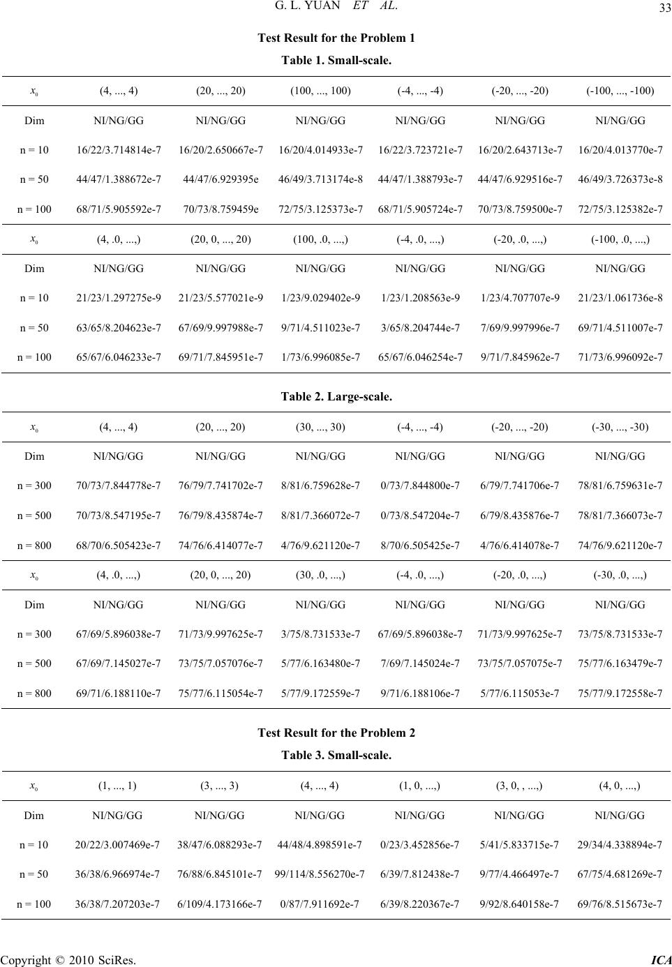

G. L. YUAN ET AL.
33
Test Result for the Problem 1
Table 1. Small-scale.
0
x
(4, ..., 4) (20, ..., 20) (100, ..., 100) (-4, ..., -4) (-20, ..., -20) (-100, ..., -100)
Dim NI/NG/GG NI/NG/GG NI/NG/GG NI/NG/GG NI/NG/GG NI/NG/GG
n = 10 16/22/3.714814e-7 16/20/2.650667e-7 16/20/4.014933e-716/22/3.723721e-7 16/20/2.643713e-7 16/20/4.013770e-7
n = 50 44/47/1.388672e-7 44/47/6.929395e 46/49/3.713174e-844/47/1.388793e-744/47/6.929516e-7 46/49/3.726373e-8
n = 100 68/71/5.905592e-7 70/73/8.759459e 72/75/3.125373e-768/71/5.905724e-770/73/8.759500e-7 72/75/3.125382e-7
0
x
(4, .0, ...,) (20, 0, ..., 20) (100, .0, ...,) (-4, .0, ...,) (-20, .0, ...,) (-100, .0, ...,)
Dim NI/NG/GG NI/NG/GG NI/NG/GG NI/NG/GG NI/NG/GG NI/NG/GG
n = 10 21/23/1.297275e-9 21/23/5.577021e-9 1/23/9.029402e-9 1/23/1.208563e-9 1/23/4.707707e-9 21/23/1.061736e-8
n = 50 63/65/8.204623e-7 67/69/9.997988e-7 9/71/4.511023e-7 3/65/8.204744e-7 7/69/9.997996e-7 69/71/4.511007e-7
n = 100 65/67/6.046233e-7 69/71/7.845951e-7 1/73/6.996085e-7 65/67/6.046254e-7 9/71/7.845962e-7 71/73/6.996092e-7
Table 2. Large-scale.
0
x
(4, ..., 4) (20, ..., 20) (30, ..., 30) (-4, ..., -4) (-20, ..., -20) (-30, ..., -30)
Dim NI/NG/GG NI/NG/GG NI/NG/GG NI/NG/GG NI/NG/GG NI/NG/GG
n = 300 70/73/7.844778e-7 76/79/7.741702e-7 8/81/6.759628e-7 0/73/7.844800e-7 6/79/7.741706e-7 78/81/6.759631e-7
n = 500 70/73/8.547195e-7 76/79/8.435874e-7 8/81/7.366072e-7 0/73/8.547204e-7 6/79/8.435876e-7 78/81/7.366073e-7
n = 800 68/70/6.505423e-7 74/76/6.414077e-7 4/76/9.621120e-7 8/70/6.505425e-7 4/76/6.414078e-7 74/76/9.621120e-7
0
x
(4, .0, ...,) (20, 0, ..., 20) (30, .0, ...,) (-4, .0, ...,) (-20, .0, ...,) (-30, .0, ...,)
Dim NI/NG/GG NI/NG/GG NI/NG/GG NI/NG/GG NI/NG/GG NI/NG/GG
n = 300 67/69/5.896038e-7 71/73/9.997625e-7 3/75/8.731533e-767/69/5.896038e-7 71/73/9.997625e-7 73/75/8.731533e-7
n = 500 67/69/7.145027e-7 73/75/7.057076e-7 5/77/6.163480e-77/69/7.145024e-773/75/7.057075e-7 75/77/6.163479e-7
n = 800 69/71/6.188110e-7 75/77/6.115054e-7 5/77/9.172559e-7 9/71/6.188106e-7 5/77/6.115053e-7 75/77/9.172558e-7
Test Result for the Problem 2
Table 3. Small-scale.
0
x
(1, ..., 1) (3, ..., 3) (4, ..., 4) (1, 0, ...,) (3, 0, , ...,) (4, 0, ...,)
Dim NI/NG/GG NI/NG/GG NI/NG/GG NI/NG/GG NI/NG/GG NI/NG/GG
n = 10 20/22/3.007469e-7 38/47/6.088293e-7 44/48/4.898591e-70/23/3.452856e-75/41/5.833715e-7 29/34/4.338894e-7
n = 50 36/38/6.966974e-7 76/88/6.845101e-7 99/114/8.556270e-76/39/7.812438e-79/77/4.466497e-7 67/75/4.681269e-7
n = 100 36/38/7.207203e-7 6/109/4.173166e-7 0/87/7.911692e-76/39/8.220367e-79/92/8.640158e-7 69/76/8.515673e-7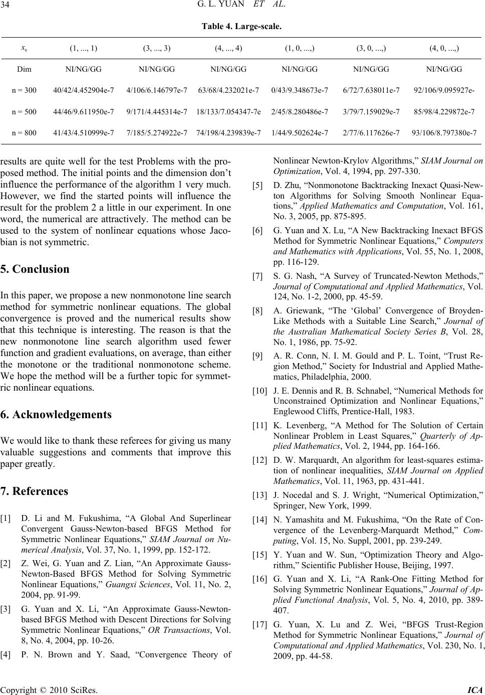

G. L. YUAN ET AL.
34
Table 4. Large-scale.
0
x
(1, ..., 1) (3, ..., 3) (4, ..., 4) (1, 0, ...,) (3, 0, ...,) (4, 0, ...,)
Dim NI/NG/GG NI/NG/GG NI/NG/GG NI/NG/GG NI/NG/GG NI/NG/GG
n = 300 40/42/4.452904e-7 4/106/6.146797e-7 63/68/4.232021e-70/43/9.348673e-7 6/72/7.638011e-7 92/106/9.095927e-
n = 500 44/46/9.611950e-7 9/171/4.445314e-7 18/133/7.054347-7e 2/45/8.280486e-73/79/7.159029e-7 85/98/4.229872e-7
n = 800 41/43/4.510999e-7 7/185/5.274922e-7 74/198/4.239839e-7 1/44/9.502624e-72/77/6.117626e-7 93/106/8.797380e-7
results are quite well for the test Problems with the pro-
posed method. The initial points and the dimension don’t
influence the performance of the algorithm 1 very much.
However, we find the started points will influence the
result for the problem 2 a little in our experiment. In one
word, the numerical are attractively. The method can be
used to the system of nonlinear equations whose Jaco-
bian is not symmetric.
5. Conclusion
In this paper, we propose a new nonmonotone line search
method for symmetric nonlinear equations. The global
convergence is proved and the numerical results show
that this technique is interesting. The reason is that the
new nonmonotone line search algorithm used fewer
function and gradient evaluations, on average, than either
the monotone or the traditional nonmonotone scheme.
We hope the method will be a further topic for symmet-
ric nonlinear equations.
6. Acknowledgements
We would like to thank these referees for giving us many
valuable suggestions and comments that improve this
paper greatly.
7. References
[1] D. Li and M. Fukushima, “A Global And Superlinear
Convergent Gauss-Newton-based BFGS Method for
Symmetric Nonlinear Equations,” SIAM Journal on Nu-
merical Analysis, Vol. 37, No. 1, 1999, pp. 152-172.
[2] Z. Wei, G. Yuan and Z. Lian, “An Approximate Gauss-
Newton-Based BFGS Method for Solving Symmetric
Nonlinear Equations,” Guangxi Sciences, Vol. 11, No. 2,
2004, pp. 91-99.
[3] G. Yuan and X. Li, “An Approximate Gauss-Newton-
based BFGS Method with Descent Directions for Solving
Symmetric Nonlinear Equations,” OR Transactions, Vol.
8, No. 4, 2004, pp. 10-26.
[4] P. N. Brown and Y. Saad, “Convergence Theory of
Nonlinear Newton-Krylov Algorithms,” SIAM Journal on
Optimization, Vol. 4, 1994, pp. 297-330.
[5] D. Zhu, “Nonmonotone Backtracking Inexact Quasi-New-
ton Algorithms for Solving Smooth Nonlinear Equa-
tions,” Applied Mathematics and Computation, Vol. 161,
No. 3, 2005, pp. 875-895.
[6] G. Yuan and X. Lu, “A New Backtracking Inexact BFGS
Method for Symmetric Nonlinear Equations,” Computers
and Mathematics with Applications, Vol. 55, No. 1, 2008,
pp. 116-129.
[7] S. G. Nash, “A Survey of Truncated-Newton Methods,”
Journal of Computational and Applied Mathematics, Vol.
124, No. 1-2, 2000, pp. 45-59.
[8] A. Griewank, “The ‘Global’ Convergence of Broyden-
Like Methods with a Suitable Line Search,” Journal of
the Australian Mathematical Society Series B, Vol. 28,
No. 1, 1986, pp. 75-92.
[9] A. R. Conn, N. I. M. Gould and P. L. Toint, “Trust Re-
gion Method,” Society for Industrial and Applied Mathe-
matics, Philadelphia, 2000.
[10] J. E. Dennis and R. B. Schnabel, “Numerical Methods for
Unconstrained Optimization and Nonlinear Equations,”
Englewood Cliffs, Prentice-Hall, 1983.
[11] K. Levenberg, “A Method for The Solution of Certain
Nonlinear Problem in Least Squares,” Quarterly of Ap-
plied Mathematics, Vol. 2, 1944, pp. 164-166.
[12] D. W. Marquardt, An algorithm for least-squares estima-
tion of nonlinear inequalities, SIAM Journal on Applied
Mathematics, Vol. 11, 1963, pp. 431-441.
[13] J. Nocedal and S. J. Wright, “Numerical Optimization,”
Springer, New York, 1999.
[14] N. Yamashita and M. Fukushima, “On the Rate of Con-
vergence of the Levenberg-Marquardt Method,” Com-
puting, Vol. 15, No. Suppl, 2001, pp. 239-249.
[15] Y. Yuan and W. Sun, “Optimization Theory and Algo-
rithm,” Scientific Publisher House, Beijing, 1997.
[16] G. Yuan and X. Li, “A Rank-One Fitting Method for
Solving Symmetric Nonlinear Equations,” Journal of Ap-
plied Functional Analysis, Vol. 5, No. 4, 2010, pp. 389-
407.
[17] G. Yuan, X. Lu and Z. Wei, “BFGS Trust-Region
Method for Symmetric Nonlinear Equations,” Journal of
Computational and Applied Mathematics, Vol. 230, No. 1,
2009, pp. 44-58.

G. L. YUAN ET AL.
35
[18] G. Yuan, S. Meng and Z. Wei, “A Trust-Region-Based
BFGS Method with Line Search Technique for Symmet-
ric Nonlinear Equations,” Advances in Operations Re-
search, Vol. 2009, 2009, pp. 1-20.
[19] G. Yuan, Z. Wang and Z. Wei, “A Rank-One Fitting
Method with Descent Direction for Solving Symmetric
Nonlinear Equations,” International Journal of Commu-
nications, Network and System Sciences, Vol. 2, No. 6,
2009, pp. 555-561.
[20] G. Yuan, Z. Wei and X. Lu, “A Nonmonotone Trust Re-
gion Method for Solving Symmetric Nonlinear Equa-
tions,” Chinese Quarterly Journal of Mathematics, Vol.
24, No. 4, 2009, pp. 574-584.
[21] H. Zhang and W. Hager, “A Nonmonotone Line Search
Technique and Its Application to Unconstrained Optimi-
zation,” SIAM Journal on Optimization, Vol. 14, No. 4,
2004, pp. 1043-1056.
[22] J. M. Ortega and W. C. Rheinboldt, “Iterative Solution of
Nonlinear Equations in Several Variables,” Academic
Press, New York, 1970.
[23] E. Yamakawa and M. Fukushima, “Testing Parallel Bari-
able Transformation,” Computational Optimization and
Applications, Vol. 13, 1999, pp. 253-274.