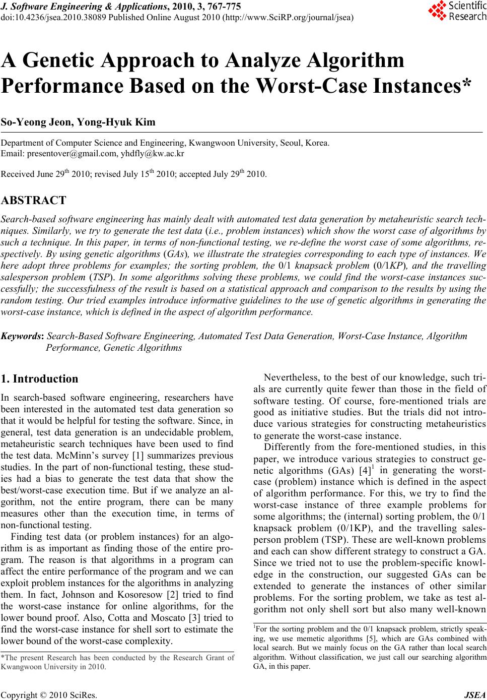
J. Software Engineering & Applications, 2010, 3, 767-775
doi:10.4236/jsea.2010.38089 Published Online August 2010 (http://www.SciRP.org/journal/jsea)
767
A Genetic Approach to Analyze Algorithm
Performance Based on the Worst-Case Instances*
So-Yeong Jeon, Yong-Hyuk Kim
Department of Computer Science and Engineering, Kwangwoon University, Seoul, Korea.
Received June 29th 2010; revised July 15th 2010; accepted July 29th 2010.
ABSTRACT
Search-based software engineering has mainly dealt with automated test data generation by metaheuristic search tech-
niques. Similarly, we try to generate the test data (i.e., problem instances) which show the worst case of algorithms by
such a technique. In this paper, in terms of non-functional testing, we re-define the worst case of some algorithms, re-
spectively. By using genetic algorithms (GAs), we illustrate the strategies corresponding to each type of instances. We
here adopt three problems for examples; the sorting problem, the 0/1 knapsack problem (0/1KP), and the travelling
salesperson problem (TSP). In some algorithms solving these problems, we could find the worst-case instances suc-
cessfully; the successfulness of the result is based on a statistical approach and comparison to the results by using the
random testing. Our tried examples introduce informa tive guidelines to the use of genetic a lgorithms in generating the
worst-case instance, which is defined in the aspect of algorithm performance.
Keywords: Search-Based Software Engineering, Automated Test Data Generation, Worst-Case Instance, Algorithm
Performance, Genet i c Al go ri t hms
1. Introduction
In search-based software engineering, researchers have
been interested in the automated test data generation so
that it would be helpful for testing the software. Since, in
general, test data generation is an undecidable problem,
metaheuristic search techniques have been used to find
the test data. McMinn’s survey [1] summarizes previous
studies. In the part of non-functional testing, these stud-
ies had a bias to generate the test data that show the
best/worst-case execution time. But if we analyze an al-
gorithm, not the entire program, there can be many
measures other than the execution time, in terms of
non-functional testing.
Finding test data (or problem instances) for an algo-
rithm is as important as finding those of the entire pro-
gram. The reason is that algorithms in a program can
affect the entire performance of the program and we can
exploit problem instances for the algorithms in analyzing
them. In fact, Johnson and Kosoresow [2] tried to find
the worst-case instance for online algorithms, for the
lower bound proof. Also, Cotta and Moscato [3] tried to
find the worst-case instance for shell sort to estimate the
lower bound of the worst-case complexity.
Nevertheless, to the best of our knowledge, such tri-
als are currently quite fewer than those in the field of
software testing. Of course, fore-mentioned trials are
good as initiative studies. But the trials did not intro-
duce various strategies for constructing metaheuristics
to generate the worst-case instance.
Differently from the fore-mentioned studies, in this
paper, we introduce various strategies to construct ge-
netic algorithms (GAs) [4]1 in generating the worst-
case (problem) instance which is defined in the aspect
of algorithm performance. For this, we try to find the
worst-case instance of three example problems for
some algorithms; the (internal) sorting problem, the 0/1
knapsack problem (0/1KP), and the travelling sales-
person problem (TSP). These are well-known problems
and each can show different strategy to construct a GA.
Since we tried not to use the problem-specific knowl-
edge in the construction, our suggested GAs can be
extended to generate the instances of other similar
problems. For the sorting problem, we take as test al-
gorithm not only shell sort but also many well-known
1For the sorting problem and the 0/1 knapsack problem, strictly speak-
ing, we use memetic algorithms [5], which are GAs combined with
local search. But we mainly focus on the GA rather than local search
algorithm. Without classification, we just call our searching algorith
m
GA, in this paper.
*The present Research has been conducted by the Research Grant o
f
Kwangwoon University in 2010.

A Genetic Approach to Analyze Algorithm Performance Based on the Worst-Case Instances 768
sorting algorithms; quick sort, heap sort, merge sort,
insertion sort, and advanced quick sort. For the 0/1KP
and the TSP, we test the algorithm based on a greedy
approach, comparing to the known-optimal algorithms
which are based on the dynamic programming.
The remaining part of this paper is organized in the
following. In Section 2, we introduce GAs and the
three adopted problems with their popular algorithms.
Also we define the worst-case instance for each prob-
lem, in terms of non-functional testing. In Section 3,
we present our GAs for finding the worst-case instance.
In Section 4, we explain our experiment plan and the
results. We make conclusions in Section 5.
2. Search Technique and Three Problems
with Algorithms
2.1 Search Technique: Genetic Algorithms
The genetic algorithm (GA) [4] is a non-deterministic
algorithm. A non-deterministic algorithm makes guesses,
which may or may not be the answer of the problem the
algorithm wants to solve. So, it consists of two phases;
the guess phase and the evaluation phase. In the guess
phase, guesses are made. In the evaluation phase, those
guesses are evaluated by how close they are to the right
answer. For evaluating guesses, the objective function is
defined. This function takes a guess and returns the nu-
merical value which indicates how close the guess is to
the right answer. In other words, a deterministic algo-
rithm searches for an object which maximizing the given
objective function.
How does GA make a guess? By the principle of evo-
lution. GA manages multiple guesses or individuals. We
call the set of individual population. A new individual
can be constructed by two operations; crossover and mu-
tation. The crossover takes two individuals and returns
one new individual. This new one is made by assembling
each pattern of the two individuals. The mutation takes
one individual and returns the individual which has
slightly changed pattern from the taken individual. A
pattern is found in the representation of the individual.
Thus, the way an individual is represented is closely re-
lated to the way of making individuals. GA substitutes
new individuals for some part of the population; this op-
eration is called replacement.
How do we select individuals (in the population) for
the crossover and the mutation as the input? Which indi-
viduals should we replace? By the qualities and the fit-
nesses [4] of the individuals. These are evaluated in the
evaluation phase. The quality of an individual is the re-
turn value of the objective function. The fitness of an
individual is evaluated using some part of the population
or the entire population, as well as the individual to be
evaluated. The fitnesses (not qualities) of the individuals
are directly used to selection; fitness evaluation strategies
are designed to increase the chances that some individu-
als with low qualities are selected. Note that using only
qualities for selecting individuals can lose the diversity
of the population and narrow the search range of GAs.
Using the above operations, GA evolves the population
until given stop condition is satisfied.
On the other hand, a local search algorithm can be
combined with a GA. Given an individual, the local
search tries to find out the individual with the best qual-
ity near the given individual. A GA combined with local
search algorithms is called a memetic algorithm (MA)
[5].
Since we want to generate the worst-case instance,
each individual is a problem instance. Also, we should
define the objective function so that this function returns
the value indicating how close given individual is to the
worst case. Thus the definition of the function depends
on our definition of the worst case. Also, the way an in-
stance is represented and strategies of crossover, muta-
tion, replacement, fitness evaluation, and stop condition
should be defined.
2.2 Sorting Problem
In the sorting problem, we are given an array of elements
and their comparison operator. The correct solution of
this problem is a sorted array in ascending (or descending)
order. For the sorting problem, we assume that the com-
parison between elements takes so long time that it con-
trols the total execution time. An instance of the problem
is an array of elements to be sorted where the size of the
array is fixed. Let the worst-case instance (array) be the
instance that needs the most element-comparisons to sort.
In this paper, we will test the following well-known
sorting algorithms: quick sort, merge sort, heap sort, in-
sertion sort, shell sort, and advanced quick sort.
Quick sort and merge sort [6] use the divide-and-
conquer strategy. In the quick sort, a pivot element [6] is
typically taken as the first element in the array to be di-
vided into two partitions; we use the same method in the
tested our quick sort. Heap sort [6] mainly uses a data
structure called heap [6]. Insertion sort [6] inserts each
element of the array into the already-sorted part of the
array one by one. Shell sort [7] uses insertion sort re-
peatedly using sequence of increments [8]. In tested shell
sort, we use the sequence as the reverse order of {hn},
where n ≥ 0 and hn+1 = 3 × hn + 1 with h0 = 1, where the
sequence is bounded above the size of sorted array. To
improve the quick sort, the advanced quick sort [6] takes
as a pivot element the median element of three elements
which are randomly chosen from the array to be divided
into partitions.
2.3 Zero/One Knapsack Problem
Let itemi be an ordered pair vi , wi where vi is its value
and wi is its weight. For a given set S = {item1, item2, …,

A Genetic Approach to Analyze Algorithm Performance Based on the Worst-Case Instances 769
itemn}, we want to put items in S into the knapsack where
the maximum capacity W is given as cw × ∑wi where i=1,
2, ..., n. Here cw  (0, 1) is called the weight coefficient.
The optimal solution of the problem is the subset A of S
such that ∑ vi (itemi  A) is maximized and ∑ wi  W
(itemi  A), where ∑ vi (itemi  A) is called the objective
value.
An algorithm based on the greedy approach [9] for this
problem orders items in non-increasing order according
to the ‘value per unit weight’ or profit density. Then, it
tries to put the items in sequence satisfying that the total
weight of the knapsack does not exceed W.
We will test the above algorithm in terms of the objec-
tive value. An instance of this problem is the set S where
the size of S and cw is fixed. Let the worst-case instance
be the instance maximizing (O−P)/O, where P is the ob-
jective value obtained by the above algorithm and O is
the objective value obtained by an optimal algorithm
based on dynamic programming [9].
2.4 Travelling Salesperson Problem
A weighted, directed graph G(V, E) is given, where V =
{1, 2, ..., n} is a set of cities. An edge e(i, j)  E
weighted by cij represents that it costs cij to go from cityi
to cityj. An example is given in Figure 1. The optimal
solution for the TSP is the tour, which is a Hamiltonian
circuit of G, that takes the lowest (optimal) total cost if
the tour exists. For our test, we assume that there always
exists at least one tour although the tour is too expensive.
The graph G can be represented as an N × N adjacency
matrix as in Figure 1.
In a greedy approach we consider, we start from city1.
To make a tour, we visit the adjacent city to which we
029 100
106 4
100 708
631000
C
æö
÷
ç÷
ç÷
ç÷
ç÷
ç÷
=ç÷
÷ ç÷
ç÷
ç÷
ç÷
ç÷
ç
èø
Figure 1. Two representations of an instance for TSP.
NOTE. The cost to go from city1 to city2 is 2. This cost is the
[1, 2]-th element of the matrix C. On the other hand, the
cost to go from city2 to city1 is 1. This cost is the [2, 1]-th
element of the matrix C
can go from the current city at the lowest cost under the
restraint that the city to go has not been visited before.
Once the tour is constructed, 2-opt [10] improves this
tour. Since the given graph is directed, two tours are de-
rived from a base tour at one move in 2-opt; one derived
tour is the reverse order of the other derived tour.
We will test an algorithm which uses the greedy ap-
proach with 2-opt in terms of the objective value (the
tour cost). An instance of this problem is the graph G(V,
E) where the size of V is fixed. So, let the worst-case
instance be the instance maximizing (P−O)/O, where P is
the objective value obtained by the above algorithm and
O is the objective value obtained by an optimal algorithm
based on dynamic programming [9].
3. Genetic Algorithms
3.1 Framework and Things in Common
There exist some trials to design somewhat different GAs
[11-13] rather than just adopting traditional design. We
also adopt a non-traditional framework of GAs. In our
framework, the initialization of a population is done first.
Then the following procedure is repeated until the stop
condition we set is satisfied: 1) Fitness evaluation is done
first. 2) Two parents are selected from the population. 3)
One new individual is created by the crossover of the two
parents. The other two new individuals are created by the
local search from the mutation of each parent; one indi-
vidual from one parent and another from the other parent.
Steps 2) and 3) are repeated until sufficiently many new
individuals are created. 4) Some individuals are replaced
from the population with the new individuals.
The strategy of the population initialization, fitness
evaluation, selection, replacement, and stop condition are
fixed in our GAs. The strategies of other operations are
different for each problem; these strategies will be intro-
duced in the next sections. The initialization of the popu-
lation is based on random generation. For the fitness
evaluation, we used one based on population sharing [4].
The formula is as follows:
Fi = fi / ∑ j{1,2, ..., n} s(dij), (1)
where
 Fi is the fitness of the i-th individual,
 fi is given as (Ci − Cmin) + (Cmax − Cmin) / (k − 1),
 Ci is the quality of the i-th individual,
 Cmin is the minimum quality among individuals,
 Cmax is the maximum quality among individuals,
 k (k >1) is a selective pressure,
 n is the population size,
 s(dij) is given as 1−(dij/) ,
 dij is the distance between the i-th individual and the
j-th one, and
  is the longest distance among all dij's.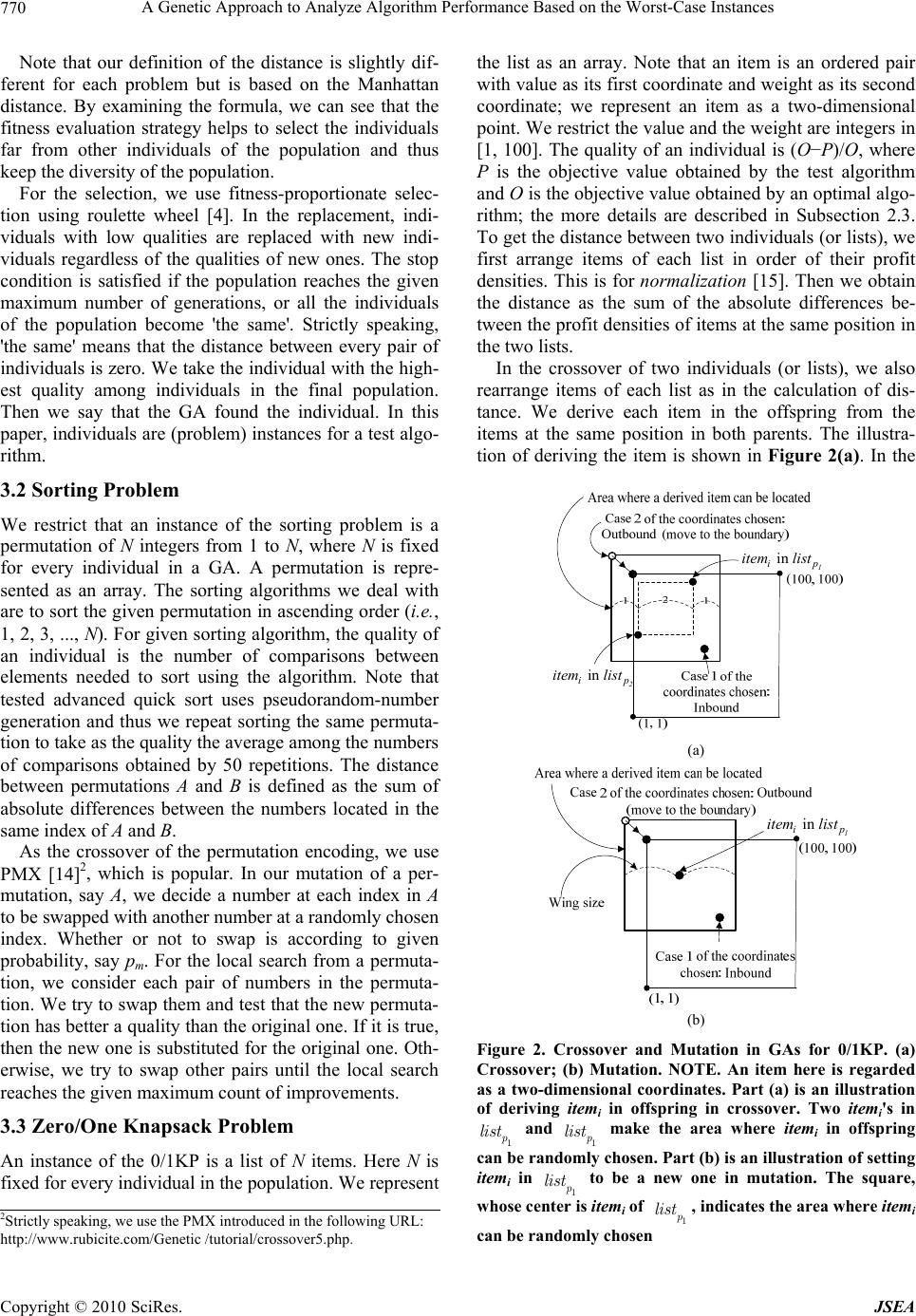

A Genetic Approach to Analyze Algorithm Performance Based on the Worst-Case Instances 770
Note that our definition of the distance is slightly dif-
ferent for each problem but is based on the Manhattan
distance. By examining the formula, we can see that the
fitness evaluation strategy helps to select the individuals
far from other individuals of the population and thus
keep the diversity of the population.
For the selection, we use fitness-proportionate selec-
tion using roulette wheel [4]. In the replacement, indi-
viduals with low qualities are replaced with new indi-
viduals regardless of the qualities of new ones. The stop
condition is satisfied if the population reaches the given
maximum number of generations, or all the individuals
of the population become 'the same'. Strictly speaking,
'the same' means that the distance between every pair of
individuals is zero. We take the individual with the high-
est quality among individuals in the final population.
Then we say that the GA found the individual. In this
paper, individuals are (problem) instances for a test algo-
rithm.
3.2 Sorting Problem
We restrict that an instance of the sorting problem is a
permutation of N integers from 1 to N, where N is fixed
for every individual in a GA. A permutation is repre-
sented as an array. The sorting algorithms we deal with
are to sort the given permutation in ascending order (i.e.,
1, 2, 3, ..., N). For given sorting algorithm, the quality of
an individual is the number of comparisons between
elements needed to sort using the algorithm. Note that
tested advanced quick sort uses pseudorandom-number
generation and thus we repeat sorting the same permuta-
tion to take as the quality the average among the numbers
of comparisons obtained by 50 repetitions. The distance
between permutations A and B is defined as the sum of
absolute differences between the numbers located in the
same index of A and B.
As the crossover of the permutation encoding, we use
PMX [14]2, which is popular. In our mutation of a per-
mutation, say A, we decide a number at each index in A
to be swapped with another number at a randomly chosen
index. Whether or not to swap is according to given
probability, say pm. For the local search from a permuta-
tion, we consider each pair of numbers in the permuta-
tion. We try to swap them and test that the new permuta-
tion has better a quality than the original one. If it is true,
then the new one is substituted for the original one. Oth-
erwise, we try to swap other pairs until the local search
reaches the given maximum count of improvements.
3.3 Zero/One Knapsack Problem
An instance of the 0/1KP is a list of N items. Here N is
fixed for every individual in the population. We represent
the list as an array. Note that an item is an ordered pair
with value as its first coordinate and weight as its second
coordinate; we represent an item as a two-dimensional
point. We restrict the value and the weight are integers in
[1, 100]. The quality of an individual is (O−P)/O, where
P is the objective value obtained by the test algorithm
and O is the objective value obtained by an optimal algo-
rithm; the more details are described in Subsection 2.3.
To get the distance between two individuals (or lists), we
first arrange items of each list in order of their profit
densities. This is for normalization [15]. Then we obtain
the distance as the sum of the absolute differences be-
tween the profit densities of items at the same position in
the two lists.
In the crossover of two individuals (or lists), we also
rearrange items of each list as in the calculation of dis-
tance. We derive each item in the offspring from the
items at the same position in both parents. The illustra-
tion of deriving the item is shown in Figure 2(a). In the
in
1
ip
item list
in 2
ip
item list
(a)
in 1
ip
item list
(b)
Figure 2. Crossover and Mutation in GAs for 0/1KP. (a)
Crossover; (b) Mutation. NOTE. An item here is regarded
as a two-dimensional coordinates. Part (a) is an illustration
of deriving itemi in offspring in crossover. Two itemi's in
1
and
1
make the area where itemi in offspring
can be randomly chosen. Part (b) is an illustration of setting
itemi in
1
li to be a new one in mutation. The square,
whose center is itemi of , indicates the area where itemi
can be randomly chosen
p
list p list
p
st
1
p
list
2Strictly speaking, we use the PMX introduced in the following URL:
http://www.rubicite.com/Genetic /tutorial/crossover5.php.

A Genetic Approach to Analyze Algorithm Performance Based on the Worst-Case Instances 771
mutation from an individual, the probability of changing
each item in the individual to be new one is pm. Once an
item is determined to be changed, we determine the area
of the square where the point indicating a new item can
be located. The center of the square is the point indicat-
ing the original item. The edge length of the square is
determined using the following probability weight func-
tion of wing size or (edge length)/2: y = a × (x − x1) + y1,
where a < 0 , y is the probability weight of choosing x as
a wing size, y1 is the probability weight of choosing x1,
and x1 is the maximum wing size. We set y1 to be 1 and
set x1 to be floor((UB −LB)/2), with UB = 100 and LB = 1.
For a given wing size, the illustration of the changing an
item to be a new one is shown in Figure 2(b).
In the local search from an individual (or a list), we try
to slightly move each item in the list and test that the new
list has a better quality than old one. If it is true, then the
new one is substituted for the original one. Otherwise, we
try to move the next item in the list. The way of slightly
moving the item (v, w) is as follows: moving to (v+1, w),
(v−1, w), (v, w+1), (v, w−1), (v+1, w+1), (v−1, w−1),
(v+1, w−1), or (v−1, w+1), excluding one out of the
boundary of [1, 100]; we take the best way among all the
possible ways.
3.4 Travelling Salesperson Problem
Every instance of the TSP is represented as an N × N
adjacency matrix. The N, which is the number of cities, is
fixed for every individual in the population. The (i, j)
element of the matrix is the cost to go from cityi to cityj.
We restrict that every element of the matrix is an integer
in [1, 100]. The TSP does not limit the values to be inte-
gers. But the bounds reduce the time for finding the
worst case, which is still helpful. We will try to find the
worst-case instance for two different versions of the
problem. In one version, the input instance G is always
represented as a symmetric matrix. In the other version,
G may be represented as an asymmetric matrix. The dis-
tance between two individuals is the sum of absolute
differences between (i, j) elements of two matrices. The
quality of an individual is (P−O)/O, where P and O are
described in Subsection 2.4.
For the crossover of two matrices, we use geographic
crossover [16-18]. The geographic crossover can gener-
ate sufficiently diverse offspring with moderate difficulty
in implementing. For the mutation from an individual (or
a matrix), our approach is to move each (i, j) element of
the matrix with given probability pm. We regard an ele-
ment as a point on the number line. If an element is
decided to be moved, the element can be moved ran-
domly within the interval whose center is the original
element. The interval size is decided by the probability
weight function of the size. The function is quite similar
to one in the 0/1KP. The small size is taken more often
than the big one. If we take large interval and the ele-
ment moves out of [1, 100], we adjust the location to
the closest boundary of the interval. We do not use the
local search here.
4. Experimental Results
Using the framework and the strategies explained in Sec-
tion 3, we tried to find the worst-case instances of test
algorithms. We used the computer of which CPU model
is Intel Core2 Duo T8100 @ 2.10 GHz. In Table 1, we
show the parameters in common for every GA. The us-
age of the mutation probability (pm) in Table 1 is de-
scribed in Subsections 3.2, 3.3, and 3.4 respectively for
the three test problems. Table 2 shows parameters in
common for every random testing [1]. We ran the same
GA fifty times to check whether our GAs are stochasti-
cally reliable. We say that two GAs are the same if and
only if they are for the same problem and they belong to
the same classification; we propose the classification in
Tables 3-5, respectively for each problem. The weight
coefficient in Table 4 is described in Subsection 2.3. The
probability weight function of wing size in the same table
is described in Subsection 3.3. The probability weight
function in Table 5 is similar to one in Table 4. This
function is referred to in Subsection 3.4.
Table 1. Parameters in common for every GA
Maximum number of generations 1,000
Selective pressure 3
# of individuals to be replaced for the next generation 30
Population size 100
Mutation probability pm 0.15
# of independent runs of GA 50
Table 2. Parameters in common for every random testing
# of instances randomly generated 30,000
# of independent runs of the random testing 50
Table 3. Classification and parameters of GAs for algo-
rithms solving sorting problem
Size of permutations:
10, 20, 30, or 40
(For advanced quick sort, we tested
only on size 10 and 20.)
Classification basis
Sorting algorithm:
quick sort, merge sort, heap sort, in-
sertion sort, shell sort, or advanced
quick sort
Elements of permutation {1,2, ..., N}
Limitation of improvement
counts in local search
The smallest integer bigger than or
equal to N×0.25+
1k
n
C
(denotes the combination.)
k
n
C

A Genetic Approach to Analyze Algorithm Performance Based on the Worst-Case Instances 772
Table 4. Classification and parameters of GAs for algo-
rithms solving 0/1KP
# of given items: 10, 20, or
30
Classification basis Weight coefficient cw:
0.25, 0.5, or 0.75
Range of value and weight of items Integers in [1, 100]
Tangent slope of probability function
of wing size.
−1 (wing size is an integer
from 1 to 50)
Table 5. Classification and parameters of GAs for algo-
rithms solving TSP
# of cities: 5 or 10
Classification basis Kind of instances: symmetric
matrix or general matrix
Range of weighted cost Integers in [1, 100]
Tangent slope of probability
function of interval size in
mutation.
−1 (interval size is an integer
from 1 to 50)
# of cutting lines in a crossover 0.5× (# of cities)
NOTE. The crossover here is geographic crossover, which uses
cutting lines.
After the run of a GA, we find one instance that shows
the maximum quality in the final population; this in-
stance is the closest to the worst case which we defined.
Among those maximum qualities which are found by
repeating the same GA fifty times, we get the average
and the standard deviation. These values are in Figure 3,
Figure 4, and Figure 5 respectively for each problem.
Those figures are represented by the histogram with error
bars; the length of error bar is 2 times the corresponding
standard deviation. Some error bars in the figures are not
identified because the corresponding standard deviation
is close to 0. Note that in the figures, ‘Avg’ means the
average, ‘Std’ means the standard deviation, ‘Random’
means the random testing method. In Figure 3, ‘Ascend’
means the permutation in ascending order (i.e., 1, 2, 3,
4, ..., N) and ‘Descend’ means the permutation in de-
scending order (i.e., N, N−1, ..., 4, 3, 2, 1). In Figure 5,
‘symmetric TSP’ means the TSP which does not allow
any problem instance with an asymmetric matrix repre-
sentation whereas ‘general TSP’ means the TSP which
allows such problem instances. The CPU seconds taken
by a run of the GA for each classification are given in
Table 6, Table 7, and Table 8, respectively for each
problem.
For test sorting algorithms, the quality of an individual
(a permutation) was defined as the number of compari-
sons between elements when the permutation is sorted
using the algorithm. In Figure 3, the worst cases of our
quick sort, insertion sort, and advance quick sort takes
more element comparisons than those of other test sort-
ing algorithms. But seeing the result when the sorting
0
10
20
30
40
50
60
70
Quick Merge Heap Insertion Shell Adv.Qui ck
Quality
Size of Permutation: 10
GA(Avg) Random(Avg) Ascend Des cen d
(a)
0
50
100
150
200
250
Quick Merge Heap Insertion Shell Adv.Qui ck
Qua l it y
Size of Permutation: 20
(b)
0
50
100
150
200
250
300
350
400
450
500
Quick Merge Heap Insertion Sh ell
Qua lit y
Size of Permutation: 30
(c)
0
100
200
300
400
500
600
700
800
900
Quick Merge Heap Insertion Shell
Quality
Size of Permutation: 40
(d)
Figure 3. Quality of the worst-case instances (sorting
problem). (a) Size of Permutation: 10; (b) Size of
Permutation: 20; (c) Size of Permutation: 30; (d) Size of
Permutation: 40. NOTE. The definition of the quality of an
instance is given in Subsection 3.2

A Genetic Approach to Analyze Algorithm Performance Based on the Worst-Case Instances 773
0.1
0.2
0.3
0.4
0.5
0.6
0.7
0.8
0.9
1
1.1
0.25 0.5 0.75
Quality
Wei
g
ht coefficient
# of Items: 10
GA(Avg) Ran dom (Avg)
(a)
0
0.1
0.2
0.3
0.4
0.5
0.6
0.7
0.25 0.5 0.75
Quality
Wei
g
ht coefficient
# of Items: 20
(b)
0
0.05
0.1
0.15
0.2
0.25
0.3
0.25 0.5 0.75
Quality
Wei
g
ht coefficient
# of Items: 30
(c)
Figure 4. Quality of the worst-case instances (0/ 1KP). (a) The
number of given items: 10; (b) The num ber of given items: 20;
(c) The number of given items: 30. NOTE. The definition of
the quality of an in st ance is given in Subsection 3.3
Table 6. CPU seconds taken by a GA for each classification
(sorting problem)
Sorting algorithm / Size
of permutations 10 20 30 40
Quick 16 75 214 456
Merge 20 122 415 1,059
Heap 19 123 414 1,093
Insertion 19 134 496 1,359
Shell 17 85 282 729
Advanced Quick 1,352 12,502 N/A N/A
0
2
4
6
8
10
12
14
16
18
510
Quality
# of cities
Symmetr ic
GA(Avg)Random(Avg)
(a)
0
5
10
15
20
25
30
35
40
510
Qual ity
# of cities
Gener a l
(b)
Figure 5. Quality of the worst-case instances (TSP). (a) The
symmetric TSP; (b) The general TSP. NOTE. The defi-
nition of the quality of an instance is given in Subsection 3.4
Table 7. CPU seconds taken by a GA for each classification
(0/1KP)
Weight coefficient / # of
given items 10 20 30
0.25 70 607 2,415
0.5 75 904 5,520
0.75 105 1,927 6,000
Table 8. CPU seconds taken by a GA for each classification
(TSP)
# of cities /
Kind of instances
Symmetric
matrix
General
matrix
5 18 18
10 472 470
permutation’s size is 10 to 20, we can predict that as the
permutation size grows, the worst-case of our advanced
quick sort takes fewer comparisons than that of our quick
sort and insertion sort. On the other hand, the worst cases
of merge sort, heap sort, and shell sort takes fewer com-
parisons than those of other algorithms.
For our test algorithm solving the 0/1KP (i.e., the al-
gorithm based on a greedy approach which we explained
in Subsection 2.3), the quality of an individual is
(O−P)/O, where P is the objective value obtained by the
test algorithm and O is the objective value obtained by an
optimal algorithm. Regardless of the number of items

A Genetic Approach to Analyze Algorithm Performance Based on the Worst-Case Instances 774
(i.e., the magnitude of the searching space), the upper
bound of the qualities is 1. We can see the result in Fig-
ure 4. For the same number of items, the higher the
weight coefficient is, the lower the average quality of the
worst cases found by our GA was. For the same coeffi-
cient, the more the given number of items is, the lower
the average quality of the worst cases found by our GA
was. When 10 items are given, the average quality of the
worst cases was generally more than 0.7; our test algo-
rithm is possibly not good enough in terms of optimality.
For our test algorithm solving the TSP (i.e., the algo-
rithm based on a greedy approach with 2-opt which we
explained in Subsection 2.4), the quality of an individual
is (P−O)/O, the meaning of O and P is similar to those in
the 0/1KP. By examining the formula of the quality, we
can assume that the upper bound of the qualities does not
exist. In Figure 5, on the same number of cities, the av-
erage quality of the worst case in the symmetric TSP was
lower than that of the worst case in the asymmetric TSP.
The average quality of the worst case found by our GA in
the symmetric TSP was about 14 when 10 cities are
given, whereas one found in the asymmetric TSP was
about 35 on the same condition; our test algorithm is
generally not good enough in terms of optimality.
Overall, the results found by GAs were superior to
those obtained by the random testing; we can conclude
that our GAs have some effectiveness.
5. Conclusions
There are few trials to find the worst case for testing al-
gorithms by GAs and the existing trials do not introduce
various strategies for constructing GAs. Therefore, by
taking as test examples the internal sorting problem, the
0/1KP, and the TSP with some algorithms for each, we
gave guidelines to the use of the GA in generating the
worst-case instance for an algorithm. First, we defined
the objective function of our GAs for the purpose of the
analysis. In this paper, the objective function returns the
quality of a problem instance; this quality indicates how-
close the instance is to the worst case. Next, we intro-
duced the framework of GAs and the specific strategies
for each test problem.
For the sorting problem, we adopted as test algorithm
quick sort, merge sort, heap sort, insertion sort, shell sort,
and advanced quick sort. We defined the worst-case in-
stance for a sorting algorithm as the instance that takes
the most number of the element comparisons in using the
algorithm. A problem instance can be represented as a
permutation. We here used the PMX for the crossover.
The mutation here swaps arbitrary elements in the per-
mutation.
For the 0/1KP and the TSP, we tested the algorithm
based on a greedy approach, comparing to an optimal
algorithm. We defined the worst-case instance as the
instance at which the test algorithm shows the most dif-
ferent objective value from that obtained by the optimal
algorithm. In the case of the 0/1KP, a problem instance
can be represented as the list of two-dimensional point
whose coordinates are integers. Our suggested crossover
is based on the idea of uniform crossover, but extended
to two-dimensional version. The mutation runs point by
point; each point in the list is moved to another close
point with a high probability or to another far point with
a low probability. In the case of the TSP, we represent a
problem instance as a square matrix. We used the geo-
graphic crossover for the representation. The mutation
runs element by element in the given matrix. Although
the element here is just a scalar (not the two-dimensional
point), the idea of mutation is similar to that of mutation
for the 0/1KP.
For the test algorithms, our GAs has some effective-
ness as the experimental results are superior to those ob-
tained by the random testing. The results of finding the
worst cases show the following: 1) At the worst case,
merge sort, heap sort, and shell sort takes fewer com-
parisons than other sorting algorithm. 2) Our greedy ap-
proach is not good enough in terms of optimality.
Our guidelines can help to analyze algorithms and can
be used to test software. Since our guidelines are just for
using GAs, we suggest giving guidelines for using other
metaheuristics to generate the worst cases. Also note that
many essential parts are still remained to analyze the
algorithms. For future work, we suggest finding some
weak points of a test algorithm and improve the algo-
rithm by analyzing the worst-case instance.
REFERENCES
[1] P. McMinn, “Search-Based Software Test Data Genera-
tion: A Survey,” Software Testing Verification And
Reliability, Vol. 14, No. 2, 2004, pp. 105-156.
[2] M. Johnson and A. Kosoresow, “Finding Worst-Case
Instances of, and Lower Bounds for, Online Algorithms
Using Genetic Algorithms,” Lecture Notes in Computer
Science, Vol. 2557, 2002, pp. 344-355.
[3] C. Cotta and P. Moscato, “A Mixed-Evolutionary Statis-
tical Analysis of an Algorithm’s Complexity,” Applied
Mathematics Letters, Vol. 16, No. 1, 2003, pp. 41-47.
[4] D. Goldberg, “Genetic Algorithms in Search, Optimi-
zation, and Machine Learning,” Kluwer Academic Publi-
shers, Boston, 1989.
[5] P. Moscato, “Memetic Algorithms: A Short Introduc-
tion,” In: D. Corne, M. Dorigo and F. Glover, Eds., New
ideas in optimization, Mcgraw-Hill, London, 1999, pp.
219-234.
[6] M. Main and W. Savitch, “Data Structures and Other
Objects Using C++,” 3rd Edtion, Pearson/Addison-
Wesley, 2004.
[7] R. Sedgewick, “Algorithms in C, Parts 1-4: Fundamentals,
Data Structures, Sorting, Searching,” 3rd Edtion,
Addison-Wesley, 1998.

A Genetic Approach to Analyze Algorithm Performance Based on the Worst-Case Instances 775
[8] D. Knuth, “The Art of Computer Programming, Volume
3: Sorting and Searching,” 2nd Edtion, Addison-Wesley,
New York, 1998.
[9] R. Neapolitan and K. Naimipour, “Foundations of
Algorithms Using C++ Pseudocode,” 3rd Edtion, Jones
and Bartlett Publishers, Inc., 2008.
[10] C. Papadimitriou and K. Steiglitz, “Combinatorial Opti-
mization: Algorithms and Complexity,” Prentice-Hall,
New Haven, 1981.
[11] L. Eshelman, “The CHC Adaptive Search Algorithm:
How to Have Safe Search When Engaging in Non-
traditional Genetic Recombination,” In: G. Rawlins, Ed.,
Foundations of Genetic Algorithms, Morgan Kauffman,
San Mateo, 1991, pp. 265-283.
[12] G. Harik, F. Lobo and D. Goldberg, “Compact Genetic
Algorithm,” IEEE Transactions on Evolutionary Compu-
tation, Vol. 3, No. 4, 1999, pp. 287-297.
[13] J. Grefenstette, “Genetic Algorithms for Changing Enviro-
nments,” Proceedings Parallel Problem Solving from
Nature, Amsterdam, Vol. 2, 1992, pp. 137-144.
[14] D. Goldberg and R. Lingle, “Alleles, Loci, and the
Traveling Salesperson Problem,” Proceedings of the
International Conference on Genetic Algorithms, Hills-
dale, 1985, pp. 154-159.
[15] S. Choi and B. Moon, “Normalization in Genetic
Algorithms,” Genetic and Evolutionary Computation—
GECCO-2003, Lecture Notes in Computer Science, Vol.
2723, Springer-Verlag, Berlin, 2003, pp. 862-873.
[16] T. Bui, B. Moon, “On Multi-Dimensional Encoding/
Crossover,” Proceedings of the 6th International Confe-
rence on Genetic Algorithms, San Francisco, 1995, pp.
49-56.
[17] B. Kahng and B. Moon, “Toward More Powerful
Recombinations,” Proceedings of the 6th International
Conference on Genetic Algorithms, San Francisco, 1995,
pp. 96-103.
[18] C. Im, H. Jung and Y. Kim, “Hybrid Genetic Algorithm
for Electromagnetic Topology Optimization,” IEEE
Transactions on Magnetics, Vol. 39, No. 1, 2003, pp.
2163-2169.