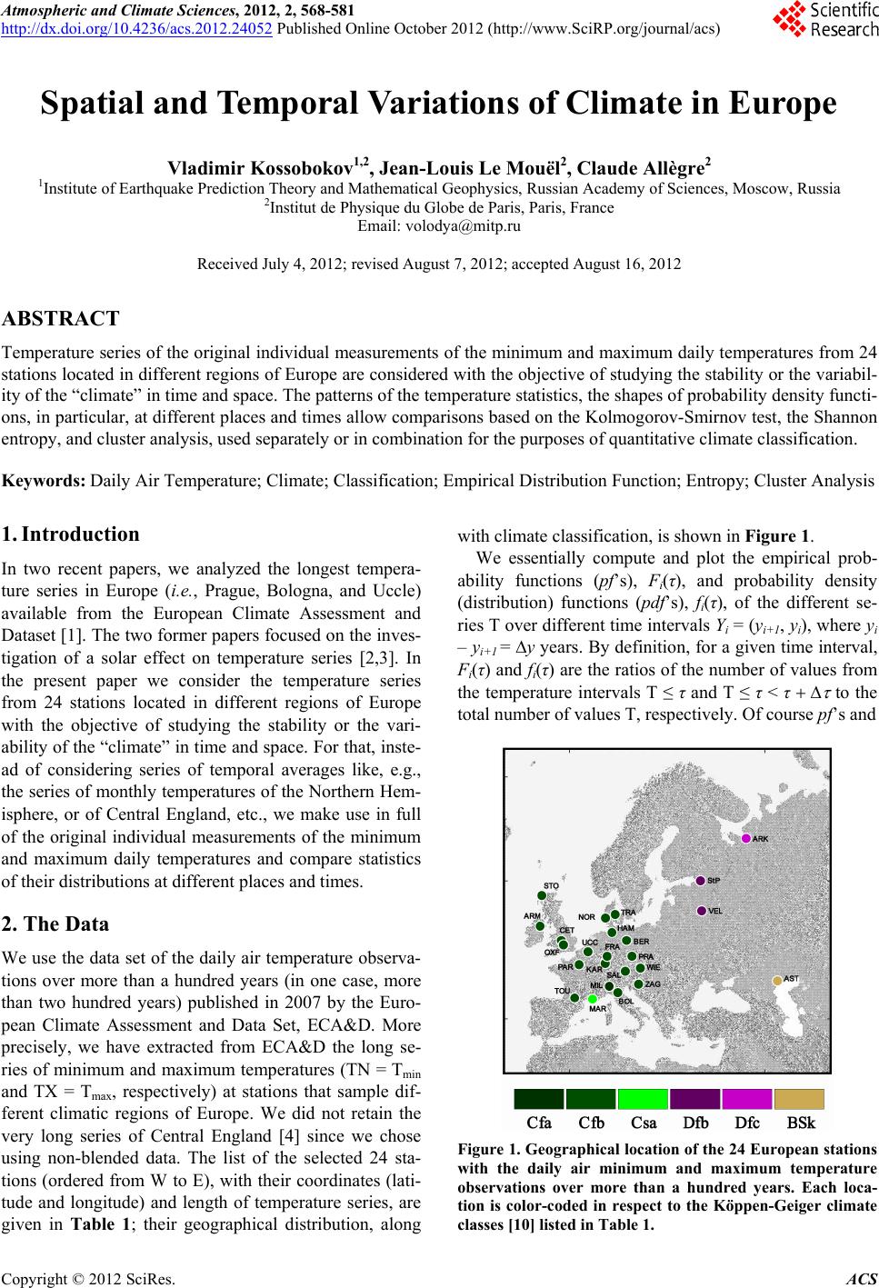
Atmospheric and Climate Sciences, 2012, 2, 568-581
http://dx.doi.org/10.4236/acs.2012.24052 Published Online October 2012 (http://www.SciRP.org/journal/acs)
Spatial and Temporal Variations of Climate in Eur ope
Vladimir Kossobokov1,2, Jean-Louis Le Mouël2, Claude Allègre2
1Institute of Earthquake Prediction Theory and Mathematical Geophysics, Russian Academy of Sciences, Moscow, Russia
2Institut de Physique du Globe de Paris, Paris, France
Received July 4, 2012; revised August 7, 2012; accepted August 16, 2012
ABSTRACT
Temperature series of the original individual measurements of the minimum and maximum daily temperatures from 24
stations located in different regions of Europe are considered with the objective of studying the stability or the variabil-
ity of the “climate” in time and space. The patterns of the temperature statistics, the shapes of probability density functi-
ons, in particular, at different places and times allow comparisons based on the Kolmogorov-Smirnov test, the Shannon
entropy, and cluster analysis, used separately or in combination for the purposes of quantitative climate classification.
Keywords: Daily Air Temperature; Climate; Classification; Empirical Distribution Function; Entropy; Cluster Analysis
1. Introduction
In two recent papers, we analyzed the longest tempera-
ture series in Europe (i.e., Prague, Bologna, and Uccle)
available from the European Climate Assessment and
Dataset [1]. The two former papers focused on the inves-
tigation of a solar effect on temperature series [2,3]. In
the present paper we consider the temperature series
from 24 stations located in different regions of Europe
with the objective of studying the stability or the vari-
ability of the “climate” in time and space. For that, inste-
ad of considering series of temporal averages like, e.g.,
the series of monthly temperatures of the Northern Hem-
isphere, or of Central England, etc., we make use in full
of the original individual measurements of the minimum
and maximum daily temperatures and compare statistics
of their distributions at different places and times.
2. The Data
We use the data set of the daily air temperature observa-
tions over more than a hundred years (in one case, more
than two hundred years) published in 2007 by the Euro-
pean Climate Assessment and Data Set, ECA&D. More
precisely, we have extracted from ECA&D the long se-
ries of minimum and maximum temperatures (TN = Tmin
and TX = Tmax, respectively) at stations that sample dif-
ferent climatic regions of Europe. We did not retain the
very long series of Central England [4] since we chose
using non-blended data. The list of the selected 24 sta-
tions (ordered from W to E), with their coordinates (lati-
tude and longitude) and length of temperature series, are
given in Table 1; their geographical distribution, along
with climate classification, is shown in Figure 1.
We essentially compute and plot the empirical prob-
ability functions (pf’s), Fi(τ), and probability density
(distribution) functions (pdf’s), fi(τ), of the different se-
ries T over different time intervals Yi = (yi+1, yi), where yi
– yi+1 = y years. By definition, for a given time interval,
Fi(τ) and fi(τ) are the ratios of the number of values from
the temperature intervals T ≤ τ and T ≤ τ < τ   to the
total number of values T, respectively. Of course pf’s and
Figure 1. Geographical location of the 24 European stations
with the daily air minimum and maximum temperature
observations over more than a hundred years. Each loca-
tion is color-coded in respect to the Köppen-Geiger climate
classes [10] listed in Table 1.
C
opyright © 2012 SciRes. ACS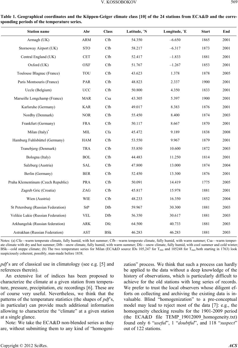

V. KOSSOBOKOV 569
Table 1. Geographical coordinates and the Köppen-Geiger climate class [10] of the 24 stations from ECA&D and the corre-
sponding periods of the temperature series.
Station name Abr Class Latitude, ˚N Longitude, ˚E Start End
Armagh (UK) ARM Cfb 54.350 –6.650 1865 2001
Stornoway Airport (UK) STO Cfb 58.217 –6.317 1873 2001
Central England (UK) CET Cfb 52.417 –1.833 1881 2001
Oxford (UK) OXF Cfb 51.767 –1.267 1853 2001
Toulouse Blagnac (France) TOU Cfb 43.623 1.378 1878 2005
Paris Montsouris (France) PAR Cfb 48.823 2.337 1900 2001
Uccle (Belgium) UCC Cfb 50.800 4.350 1833 2001
Marseille Longchamp (France) MAR Csa 43.305 5.397 1900 2001
Karlsruhe (Germany) KAR Cfb 49.017 8.383 1876 2001
Nordby (Denmark) NOR Cfb 55.450 8.400 1874 2003
Frankfurt (Germany) FRA Cfb 50.117 8.667 1870 2001
Milan (Italy)* MIL Cfa 45.472 9.189 1838 2008
Hamburg Fuhlsbüttel (Germany) HAM Cfb 53.550 9.967 1879 2001
Tranebjerg (Denmark) TRA Cfb 55.850 10.600 1872 2003
Bologna (Italy) BOL Cfb 44.483 11.250 1814 2001
Salzburg (Austria) SAL Cfb 47.800 13.000 1874 2004
Berlin (Germany) BER Cfb 52.450 13.300 1876 2001
Praha Klementinum (Czech Republic) PRA Cfb 50.091 14.419 1775 2005
Zagreb Gric (Croatia) ZAG Cfb 45.817 15.978 1881 2001
Wien (Austria) WIE Cfb 48.233 16.350 1852 2004
St Petersburg (Russian Federation) StP Dfb 59.967 30.300 1881 2003
Velikie Lukie (Russian Federation) VEL Dfb 56.350 30.617 1881 2003
Arkhangelsk (Russian federation) ARK Dfc 64.500 40.733 1881 2003
Astrakhan (Russian Federation) AST BSk 46.283 46.283 1881 2003
Notes: (a) Cfa—warm temperate climate, fully humid, with hot summer; Cfb—warm temperate climate, fully humid, with warm summer; Csa—warm temper-
ate climate with dry and hot summer; Dfb—snow climate, fully humid, with warm summer; Dfc—snow climate, fully humid, with cool summer and cold winter;
BSk—cold steppe climate; (b) The two temperature series for Milan (ECA&D source IDs 105,247 for Tmin and 105248 for Tmax both starting in 1763) look
suspiciously coherent, possibly, man-made before 1838.
pdf’s are of classical use in climatology (see e.g. [5] and
references therein).
An extensive list of indices has been proposed to
characterize the climate at a given station from tempera-
ture, pressure, precipitation, etc recordings [6]. These are
of course very useful. Nevertheless, we think that the
patterns of the temperature statistics (the shapes of pdf’s,
in particular) can provide much additional information
allowing to characterize the “climate” at a given station
at a single glance.
Note: We take the ECA&D non-blended series as they
are, without submitting them to any kind of “homogeni-
zation” process. We think that such a process can hardly
be applied to the data without a deep knowledge of the
history of observations, which is particularly difficult to
achieve for the old stations with long series of records.
We prefer to trust the local observers whose diligent ef-
forts on collecting and archiving the existing data is in-
valuable. Blind “homogenization” to a pre-conceptual
model may lead to reject most of the data [7]: e.g., the
homogeneity checking results for the 1901-2009 period
(the ECA&D file TEMP_19012009_homogeneity.txt)
found only 6 “useful”, 1 “doubtful”, and 118 “suspect”
out of 122 stations.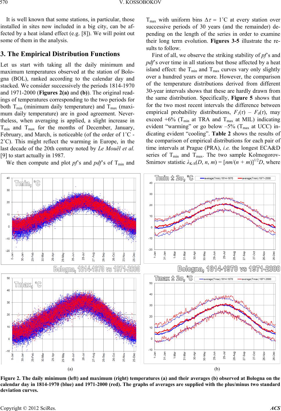

V. KOSSOBOKOV
570
It is well known that some stations, in particular, those
installed in sites now included in a big city, can be af-
fected by a heat island effect (e.g. [8]). We will point out
some of them in the analysis.
3. The Empirical Distribution Functions
Let us start with taking all the daily minimum and
maximum temperatures observed at the station of Bolo-
gna (BOL), ranked according to the calendar day and
stacked. We consider successively the periods 1814-1970
and 1971-2000 (Figures 2(a) and (b)). The original read-
ings of temperatures corresponding to the two periods for
both Tmin (minimum daily temperature) and Tmax (maxi-
mum daily temperature) are in good agreement. Never-
theless, when averaging is applied, a slight increase in
Tmin and Tmax for the months of December, January,
February, and March, is noticeable (of the order of 1˚C -
2˚C). This might reflect the warming in Europe, in the
last decade of the 20th century noted by Le Mouël et al.
[9] to start actually in 1987.
We then compute and plot pf’s and pdf’s of Tmin and
Tmax with uniform bins    1˚C at every station over
successive periods of 30 years (and the remainder) de-
pending on the length of the series in order to examine
their long term evolution. Figures 3-5 illustrate the re-
sults to follow.
First of all, we observe the striking stability of pf’s and
pdf’s over time in all stations but those affected by a heat
island effect: the Tmin and Tmax curves vary only slightly
over a hundred years or more. However, the comparison
of the temperature distributions derived from different
30-year intervals shows that these are hardly drawn from
the same distribution. Specifically, Figure 5 shows that
for the two most recent intervals the difference between
empirical probability distributions, F1(τ) – F0(τ), may
exceed +6% (Tmin at TRA and Tmax at MIL) indicating
evident “warming” or go below –5% (Tmax at UCC) in-
dicating evident “cooling”. Table 2 shows the results of
the comparison of empirical distributions for each pair of
time intervals at Prague (PRA), i.e. the longest ECA&D
series of Tmin and Tmax . The two sample Kolmogorov-
Smirnov statistic λK-S(D, n, m) = [nm/( n + m)]1/2D, where
(a) (b)
Figure 2. The daily minimum (left) and maximum (right) temperatures (a) and their averages (b) observed at Bologna on the
calendar day in 1814-1970 (blue) and 1971-2000 (red). The graphs of averages are supplied with the plus/minus two standard
deviation curves.

V. KOSSOBOKOV 571
a
b
Figure 3. The empirical probability (distribution) functions, F(τ), of the minimum (a) and maximum (b) temperatures, Tmin
and Tmax, over different time intervals. Note: the complete set of plots for the 24 European stations is given in Supplement.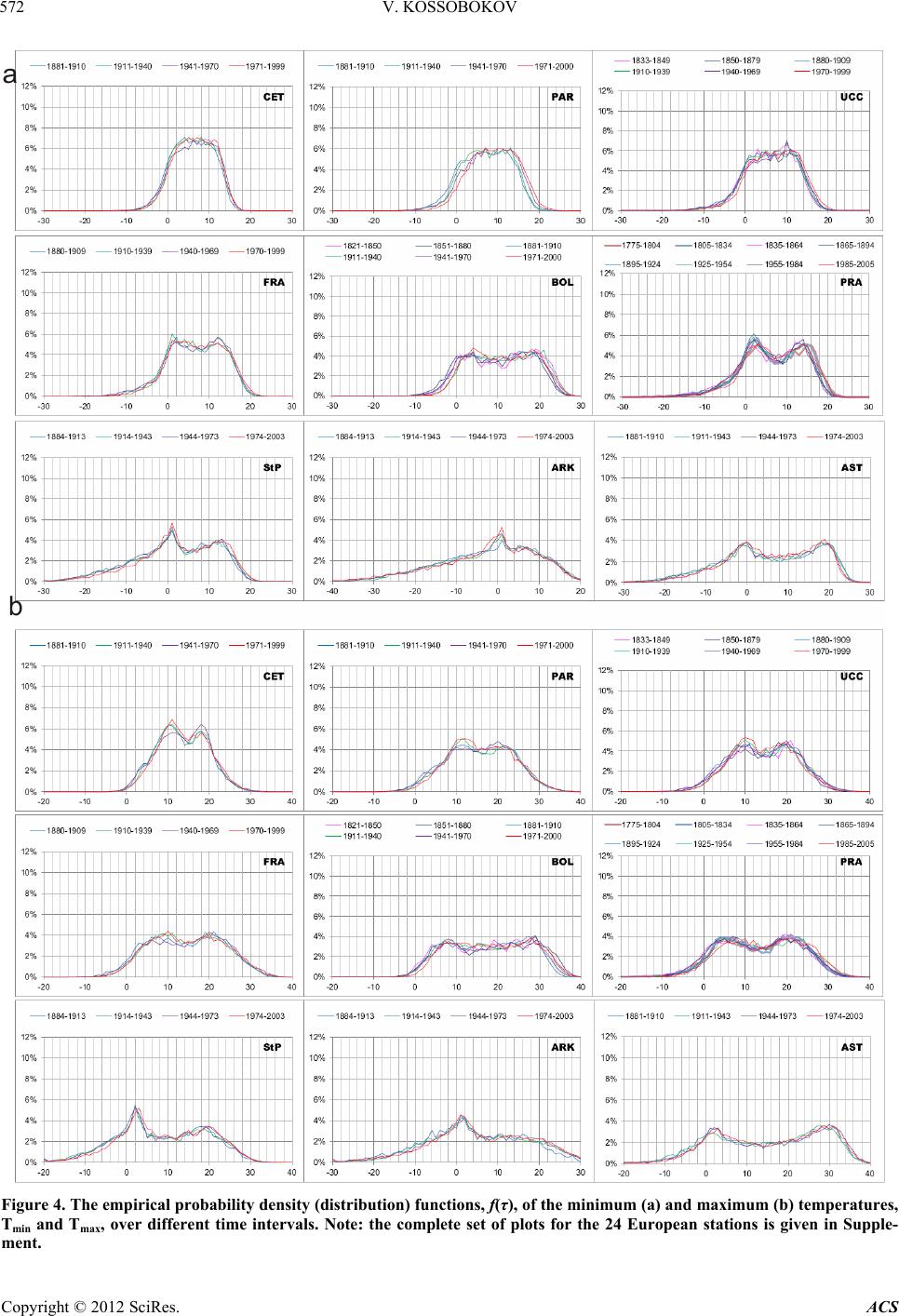

V. KOSSOBOKOV
572
a
b
Figure 4. The empirical probability density (distribution) functions, f(τ), of the minimum (a) and maximum (b) temperatures,
Tmin and Tmax, over different time intervals. Note: the complete set of plots for the 24 European stations is given in Supple-
ment.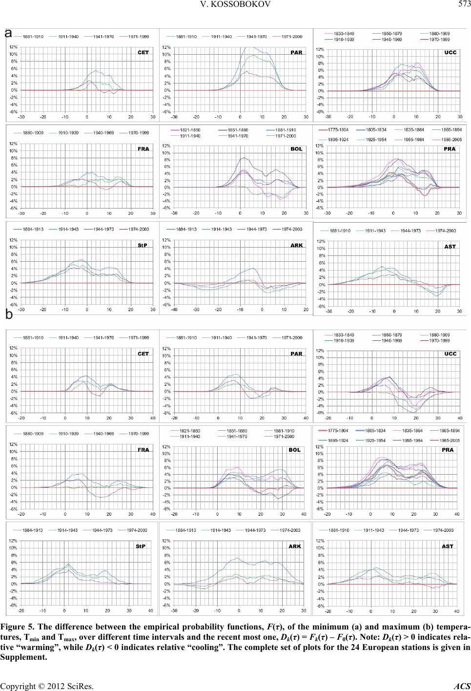

V. KOSSOBOKOV 573
a
b
Figure 5. The difference between the empirical probability functions, F(τ), of the minimum (a) and maximum (b) tempera-
tures, Tmin and Tmax, over different time intervals and the recent most one, Dk(τ) = Fk(τ) – F0(τ). Note: Dk(τ) > 0 indicates rela-
tive “warm ing”, while Dk(τ) < 0 indicates relative “cooling”. The complete set of plots for the 24 European stations is given in
Supplement.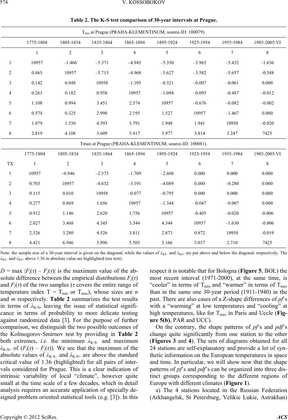

V. KOSSOBOKOV
574
Table 2. The K-S test comparison of 30-year intervals at Prague.
Tmin at Prague (PRAHA-KLEMENTINUM; source-ID: 100079).
1775-1804 1805-1834 1835-1864 1865-1894 1895-1924 1925-1954 1955-1984 1985-2005.VI
1 2 3 4 5 6 7 8
1 10957 –1.466 –5.371 –4.945 –5.350 –3.965 –5.432 –1.636
2 0.865 10957 –5.715 –4.968 –5.627 –3.582 –5.657 –0.548
3 0.142 0.048 10958 –1.105 –0.321 –0.007 –0.061 0.000
4 0.263 0.182 0.958 10957 –1.094 –0.095 –0.487 –0.012
5 1.108 0.994 3.451 2.574 10957 –0.676 –0.082 –0.002
6 0.574 0.325 2.998 2.195 1.527 10957 –1.467 0.000
7 1.879 1.530 4.593 3.791 1.948 1.941 10958 –0.020
8 2.819 4.108 5.609 5.417 3.977 3.814 3.247 7425
Tmax at Prague (PRAHA-KLEMENTINUM; source-ID: 100081).
1775-1804 1805-1834 1835-1864 1865-1894 1895-1924 1925-1954 1955-1984 1985-2005.VI
TX 1 2 3 4 5 6 7 8
1 10957 –0.946 –2.573 –1.709 –2.608 0.000 0.000 0.000
2 0.703 10957 –4.632 –3.191 –4.089 0.000 –0.280 0.000
3 0.115 0.010 10958 –0.077 –0.795 0.000 0.000 0.000
4 0.277 0.869 1.656 10957 –1.344 –0.047 –0.007 0.000
5 0.912 1.146 2.620 1.756 10957 –0.405 –0.020 -0.006
6 2.027 3.468 4.345 3.344 4.344 10957 –1.630 –0.006
7 2.326 3.280 4.526 3.811 2.873 0.872 10958 –0.019
8 4.421 6.946 5.896 5.503 5.166 3.037 2.710 7425
Note: the sample size of a 30-year interval is given on the diagonal, while the values of λKS– and λKS+ are put above and below the diagonal, respectively. The
λKS– and λKS+ above 1.36 in absolute value are highlighted (see text).
D = max |Fi(τ) – Fj(τ)| is the maximum value of the ab-
solute difference between the empirical distributions Fi(τ)
and Fj(τ) of the two samples (τ covers the entire range of
temperature index T = Tmin or Tmax), whose sizes are n
and m respectively. Table 2 summarizes the test results
in terms of λK-S, leaving the issue of statistical signifi-
cance in terms of probability to more delicate testing
against randomized data [3]. For the purpose of further
comparison, we distinguish the two possible outcomes of
the Kolmogorov-Smirnov test by providing in Table 2
both extremes, i.e. the minimum λK-S– and maximum
λK-S+ of (Fi(τ) – Fj(τ)). We see that the maximum of the
absolute values of λK-S– and λK-S+ are above the standard
critical value of 1.36 (highlighted) for all pairs of inter-
vals considered for Prague. This is a clear indication of
intrinsic variability of local “climate”, however quite
small at the time scale of a few decades, which in detail
analysis requires an accurate application of specially de-
signed problem oriented statistical tools (e.g. [3]). In this
respect it is notable that for Bologna (Figure 5, BOL) the
most recent interval (1971-2000), at the same time, is
“cooler” in terms of Tmin and “warmer” in terms of Tmax
than in the same one 30-year period (1911-1940) in the
past. There are also cases of a Z-shape differences of pf’s
with a “warming” at low temperatures and “cooling” at
high temperatures, like for Tmax in Paris and Uccle (Fig-
ure 5(b), PAR and UCC).
On the contrary, the shape patterns of pf’s and pdf’s
change quite significantly from one station to the other
(Figures 3 and 4). The sets of diagrams obtained for all
24 stations are self-explanatory and provide a lot of syn-
thetic information on the European temperatures in space
and time. In particular, we will show now that the shape
patterns of pf’s and pdf’s can be organized into three dis-
tinct groups corresponding to the different regions of
Europe with different climates (Figure 1).
a) The 4 stations located in the Russian Federation
(Arkhangelsk, St Petersburg, Velikie Lukie, Astrakhan)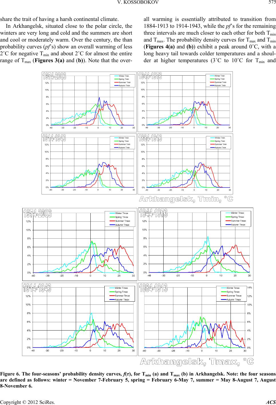

V. KOSSOBOKOV 575
share the trait of having a harsh continental climate.
In Arkhangelsk, situated close to the polar circle, the
winters are very long and cold and the summers are short
and cool or moderately warm. Over the century, the than
probability curves (pf’s) show an overall warming of less
2˚C for negative Tmin and about 2˚C for almost the entire
range of Tmax (Figures 3(a) and (b)). Note that the over-
all warming is essentially attributed to transition from
1884-1913 to 1914-1943, while the pf’s for the remaining
three intervals are much closer to each other for both Tmin
and Tmax. The probability density curves for Tmax and Tmin
(Figures 4(a) and (b)) exhibit a peak around 0˚C, with a
long heavy tail towards colder temperatures and a shoul-
der at higher temperatures (3˚C to 10˚C for Tmin and
Figure 6. The four-seasons’ probability density curves, f(τ), for Tmin (a) and Tmax (b) in Arkhangelsk. Note: the four seasons
are defined as follows: winter = November 7-February 5, spring = February 6-May 7, summer = May 8-August 7, August
8-November 6.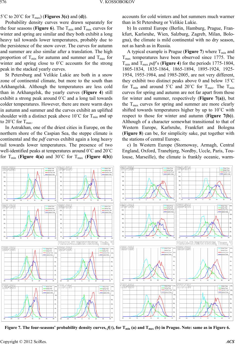

V. KOSSOBOKOV
576
5˚C to 20˚C for Tmax) (Figures 3(c) and (d)).
Probability density curves were drawn separately for
the four seasons (Figure 6). The Tmin and Tmax curves for
winter and spring are similar and they both exhibit a long
heavy tail towards lower temperatures, probably due to
the persistence of the snow cover. The curves for autumn
and summer are also similar after a translation. The high
proportion of Tmin for autumn and summer and Tmax for
winter and spring close to 0˚C accounts for the strong
peak in the stacked yearly curves.
St Petersburg and Velikie Lukie are both in a snow
zone of continental climate, but more to the south than
Arkhangelsk. Although the temperatures are less cold
than in Arkhangelsk, the yearly curves (Figure 4) still
exhibit a strong peak around 0˚C and a long tail towards
colder temperatures. However, there are more warm days
in autumn and summer and the curves exhibit an uplifted
shoulder with a distinct peak above 10˚C for Tmin and up
to 20˚C for Tmax.
In Astrakhan, one of the driest cities in Europe, on the
northern shore of the Caspian Sea, the steppe climate is
continental and the pdf curves exhibit again a long heavy
tail towards lower temperatures. The presence of two
well-identified peaks at temperatures around 0˚C and 20˚C
for Tmin (Figure 4(a) and 30˚C for Tmax (Figure 4(b))
accounts for cold winters and hot summers much warmer
than in St Petersburg or Velikie Lukie.
b) In central Europe (Berlin, Hamburg, Prague, Fran-
kfurt, Karlsruhe, Wien, Salzburg, Zagreb, Milan, Bolo-
gna), the climate is mild continental with no dry season,
not as harsh as in Russia.
A typical example is Prague (Figure 7) where Tmin and
Tmax temperatures have been observed since 1775. The
Tmin and Tmax pdf’s (Figure 4) for the periods 1775-1804,
1805-1834, 1835-1864, 1865-1894, 1895-1924, 1925-
1954, 1955-1984, and 1985-2005, are not very different,
they exhibit two distinct peaks above 0 and below 15˚C
for Tmin and around 5˚C and 20˚C for Tmax. The Tmin
curves for spring and autumn are not far apart from those
for winter and summer, respectively (Figure 7(a)), but
the Tmax curves for spring and summer are more clearly
shifted towards temperatures higher by up to 10˚C with
respect to those for winter and autumn (Figure 7(b)).
Although of a character somewhat transitional to that of
Western Europe, Karlsruhe, Frankfurt and Bologna
(Figure 8) can be, for simplicity sake, put together with
the stations of central Europe.
c) In Western Europe (Stornoway, Armagh, Central
England, Oxford, Tranebjerg, Nordby, Uccle, Paris, Tou-
louse, Marseille), the climate is frankly oceanic, warm-
Figure 7. The four-seasons’ probability density curves, f(τ), for Tmin (a) and Tmax (b) in Prague. Note: same as in Figure 6.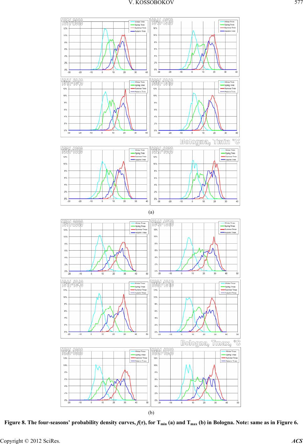

V. KOSSOBOKOV 577
(a)
(b)
Figure 8. The four-seasons’ probability density curves, f(τ), for Tmin (a) and Tmax (b) in Bologna. Note: same as in Figure 6.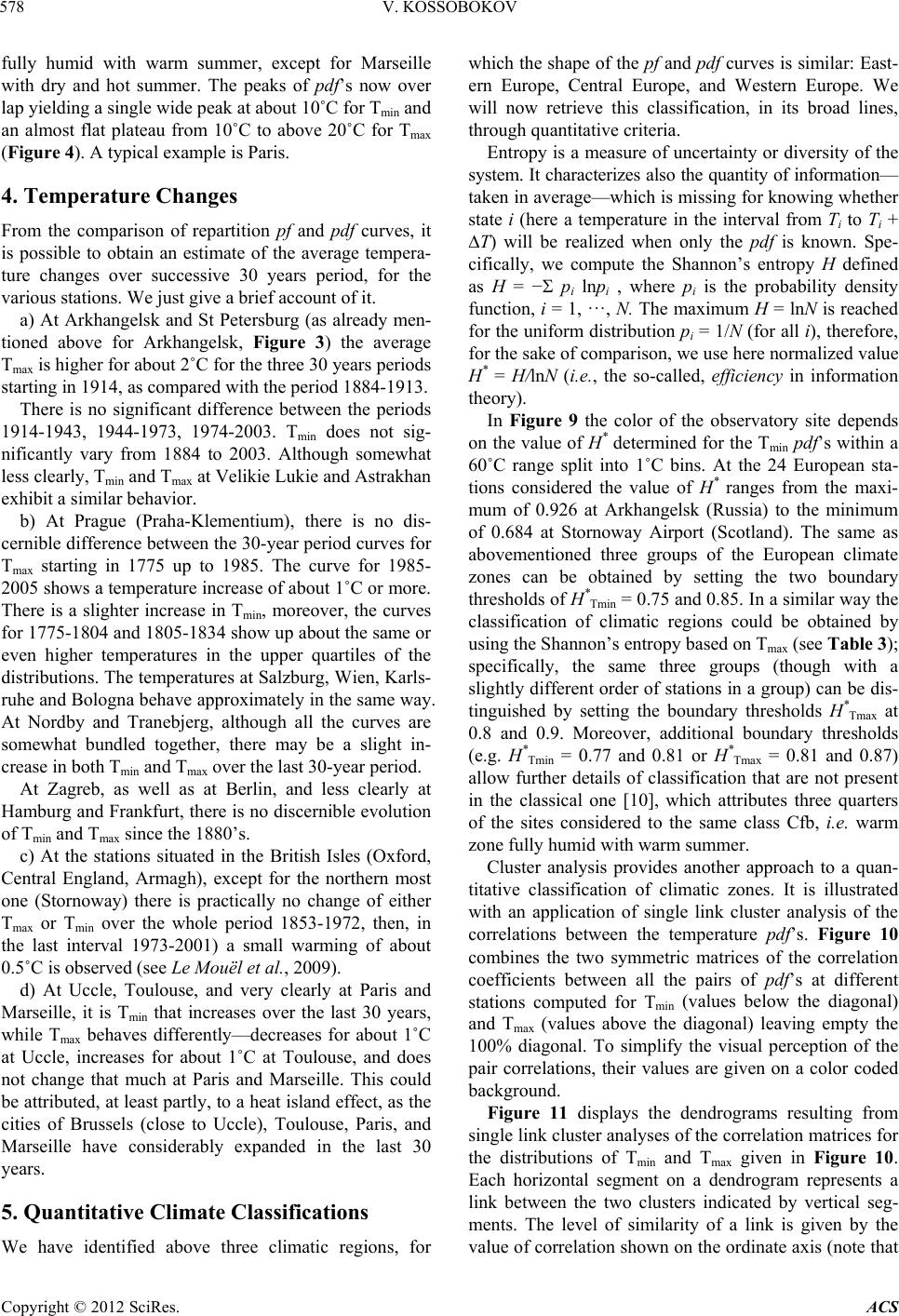

V. KOSSOBOKOV
578
fully humid with warm summer, except for Marseille
with dry and hot summer. The peaks of pdf’s now over
lap yielding a single wide peak at about 10˚C for Tmin and
an almost flat plateau from 10˚C to above 20˚C for Tmax
(Figure 4). A typical example is Paris.
4. Temperature Changes
From the comparison of repartition pf and pdf curves, it
is possible to obtain an estimate of the average tempera-
ture changes over successive 30 years period, for the
various stations. We just give a brief account of it.
a) At Arkhangelsk and St Petersburg (as already men-
tioned above for Arkhangelsk, Figure 3) the average
Tmax is higher for about 2˚C for the three 30 years periods
starting in 1914, as compared with the period 1884-1913.
There is no significant difference between the periods
1914-1943, 1944-1973, 1974-2003. Tmi n does not sig-
nificantly vary from 1884 to 2003. Although somewhat
less clearly, Tmin and Tmax at Velikie Lukie and Astrakhan
exhibit a similar behavior.
b) At Prague (Praha-Klementium), there is no dis-
cernible difference between the 30-year period curves for
Tmax starting in 1775 up to 1985. The curve for 1985-
2005 shows a temperature increase of about 1˚C or more.
There is a slighter increase in Tmin, moreover, the curves
for 1775-1804 and 1805-1834 show up about the same or
even higher temperatures in the upper quartiles of the
distributions. The temperatures at Salzburg, Wien, Karls-
ruhe and Bologna behave approximately in the same way.
At Nordby and Tranebjerg, although all the curves are
somewhat bundled together, there may be a slight in-
crease in both Tmin and Tmax over the last 30-year period.
At Zagreb, as well as at Berlin, and less clearly at
Hamburg and Frankfurt, there is no discernible evolution
of Tmin and Tmax since the 1880’s.
c) At the stations situated in the British Isles (Oxford,
Central England, Armagh), except for the northern most
one (Stornoway) there is practically no change of either
Tmax or Tmin over the whole period 1853-1972, then, in
the last interval 1973-2001) a small warming of about
0.5˚C is observed (see Le Mouël et al., 2009).
d) At Uccle, Toulouse, and very clearly at Paris and
Marseille, it is Tmin that increases over the last 30 years,
while Tmax behaves differently—decreases for about 1˚C
at Uccle, increases for about 1˚C at Toulouse, and does
not change that much at Paris and Marseille. This could
be attributed, at least partly, to a heat island effect, as the
cities of Brussels (close to Uccle), Toulouse, Paris, and
Marseille have considerably expanded in the last 30
years.
5. Quantitative Climate Classifications
We have identified above three climatic regions, for
which the shape of the pf and pdf curves is similar: East-
ern Europe, Central Europe, and Western Europe. We
will now retrieve this classification, in its broad lines,
through quantitative criteria.
Entropy is a measure of uncertainty or diversity of the
system. It characterizes also the quantity of information—
taken in average—which is missing for knowing whether
state i (here a temperature in the interval from Ti to Ti +
T) will be realized when only the pdf is known. Spe-
cifically, we compute the Shannon’s entropy H defined
as H = − pi lnpi , where pi is the probability density
function, i = 1, ···, N. The maximum H = lnN is reached
for the uniform distribution pi = 1/N (for all i), therefore,
for the sake of comparison, we use here normalized value
H* = H/lnN (i.e. , the so-called, efficiency in information
theory).
In Figure 9 the color of the observatory site depends
on the value of H* determined for the Tmin pdf’s within a
60˚C range split into 1˚C bins. At the 24 European sta-
tions considered the value of H* ranges from the maxi-
mum of 0.926 at Arkhangelsk (Russia) to the minimum
of 0.684 at Stornoway Airport (Scotland). The same as
abovementioned three groups of the European climate
zones can be obtained by setting the two boundary
thresholds of H*
Tmin = 0.75 and 0.85. In a similar way the
classification of climatic regions could be obtained by
using the Shannon’s entropy based on Tmax (see Table 3);
specifically, the same three groups (though with a
slightly different order of stations in a group) can be dis-
tinguished by setting the boundary thresholds H*
Tmax at
0.8 and 0.9. Moreover, additional boundary thresholds
(e.g. H*
Tmin = 0.77 and 0.81 or H* Tmax = 0.81 and 0.87)
allow further details of classification that are not present
in the classical one [10], which attributes three quarters
of the sites considered to the same class Cfb, i.e. warm
zone fully humid with warm summer.
Cluster analysis provides another approach to a quan-
titative classification of climatic zones. It is illustrated
with an application of single link cluster analysis of the
correlations between the temperature pdf’s. Figure 10
combines the two symmetric matrices of the correlation
coefficients between all the pairs of pdf’s at different
stations computed for Tmin (values below the diagonal)
and Tmax (values above the diagonal) leaving empty the
100% diagonal. To simplify the visual perception of the
pair correlations, their values are given on a color coded
background.
Figure 11 displays the dendrograms resulting from
single link cluster analyses of the correlation matrices for
the distributions of Tmi n and Tmax given in Figure 10.
Each horizontal segment on a dendrogram represents a
link between the two clusters indicated by vertical seg-
ments. The level of similarity of a link is given by the
value of correlation shown on the ordinate axis (note that

V. KOSSOBOKOV 579
Figure 9. The normalized Shannon’s entropy H* for Tmin (left) and Tmax (right) at the 24 European stations.
Table 3. The normalized Shannon’s entropies H* computed
from Tmin and Tmax.
Location H*Tmin H*Tmax Order by
H*Tmin and H*Tmax
STO—Stornoway airport (UK) 0.684 0.686 1 1
ARM—Armagh (UK) 0.712 0.743 2 2
CET—Central England (UK) 0.724 0.777 3 3
OXF—Oxford (UK) 0.740 0.795 4 4
PAR—Paris, (France) 0.769 0.840 5 10
MAR—Marseille (France) 0.773 0.802 6 5
UCC - Uccle (Belgium) 0.773 0.838 7 8
NOR—Nordby (Denmark) 0.779 0.817 8 6
TRA—Tranebjerg (Denmark) 0.779 0.817 9 7
TOU—Toulouse (France) 0.781 0.839 10 9
HAM—Hamburg (Germany) 0.789 0.845 11 11
FRA—Frankfurt (Germany) 0.795 0.865 12 12
KAR—Karlsruhe (Germany) 0.801 0.867 13 13
BER—Berlin (Germany) 0.806 0.870 14 14
ZAG—Zagreb Gric (Croatia) 0.820 0.879 15 19
WIE—Wien (Austria) 0.821 0.880 16 20
PRA—Prague (Czech Republic) 0.822 0.877 17 17
MIL—Milan (Italy) 0.823 0.872 18 15
SAL—Salzburg (Austria) 0.825 0.878 19 18
BOL—Bologna (Italy) 0.828 0.873 20 16
VEL—Velikie Lukie (Russia) 0.880 0.911 21 22
StP—St Petersburg (Russia) 0.886 0.906 22 21
AST—Astrakhan (Russia) 0.911 0.934 23 23
ARK—Arkhangelsk (Russia) 0.926 0.937 24 24
levels increase downwards). For example, the link, above
which a single cluster of the 24 stations is achieved, cor-
responds to a similarity level of 86.0% for Tmi n (Figure
11(a)) and 78.4% for Tmax (Figure 11(b)). For Tmin, there
are four clusters at a level of similarity above 95%: these
are Astrakhan (AST), Milan and Bologna (MIL, BOL),
Arkhangelsk (ARK), and the remaining 20 of the 24 sta-
tions. A level above 99.7% (i.e. the maximum of the
values below the diagonal in Figure 10) delivers the split
into 24 classes including each single station by breaking
the highest correlation link between Karlsruhe (KAR)
and Frankfurt (FRA). For Tmax, the level of similarity
above 90% provides separation into four clusters: these
are Astrakhan (AST), Arkhangelsk (ARK), St Petersburg
and Velikie Lukie (StP, VEL), and the remaining 20
European stations. The level of 95% splits two additional
clusters: Stornoway (STO) and Toulouse and Marseille
(TOU, MAR). A level above 99.4% (i.e. the maximum of
the values above the diagonal in Figure 10) is needed to
break all the Tmax correlation links between the 24 sta-
tions.
6. Conclusions
The study of the statistical distribution of daily minimum
and maximum temperatures in 24 European stations,
from long series of more than a century, reveals two
simple traits: a strong stability of the distributions at the
different stations during the whole time span available; a
strong, but ordered along a general trend, variability in
space.
In the Eastern European stations, one notices an in-
crease of about 2˚C of the maximum temperatures in the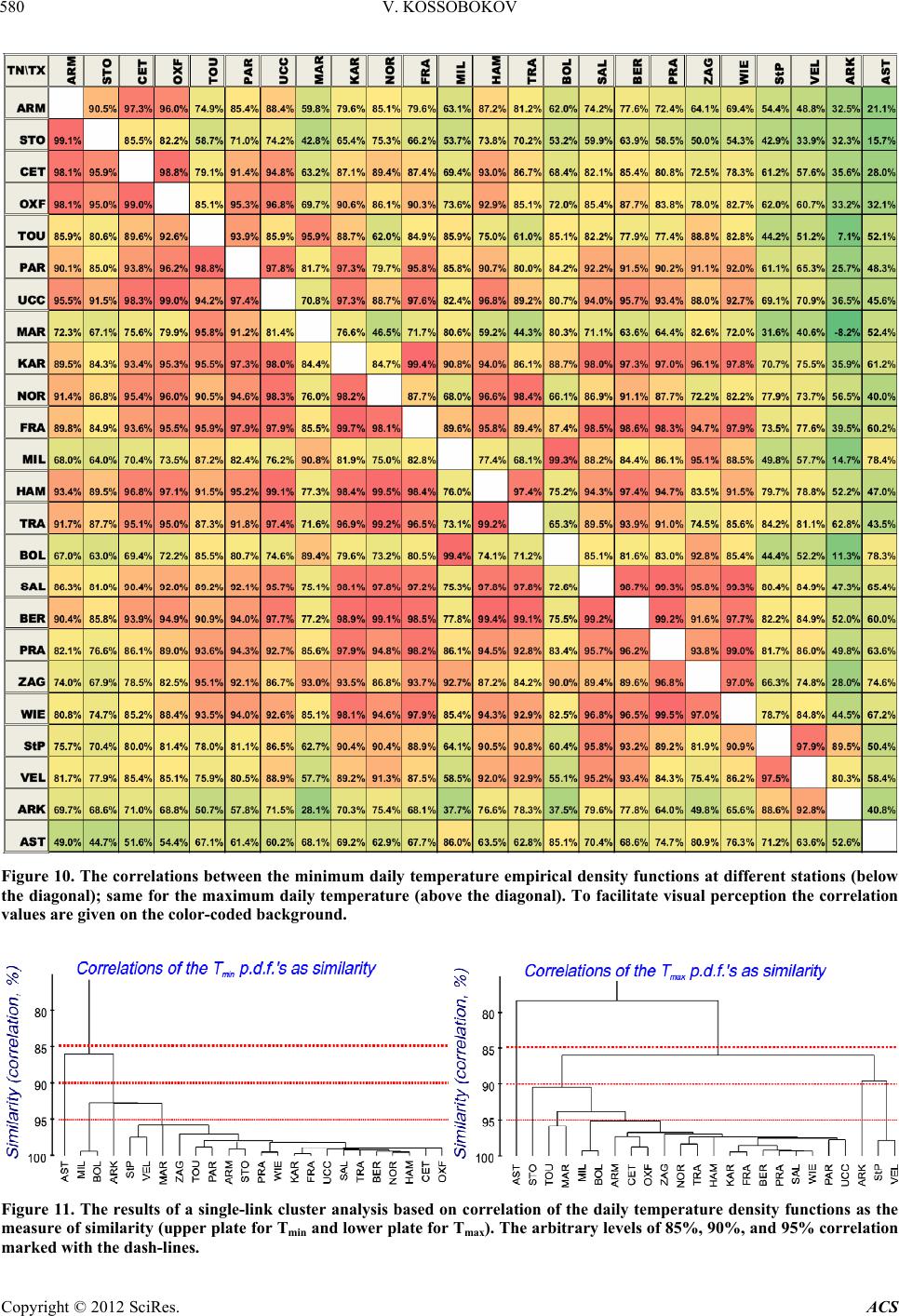

V. KOSSOBOKOV
580
Figure 10. The correlations between the minimum daily temperature empirical density functions at different stations (below
the diagonal); same for the maximum daily temperature (above the diagonal). To facilitate visual perception the correlation
values are given on the color- code d background.
Figure 11. The results of a single-link cluster analysis based on correlation of the daily temperature density functions as the
measure of similarity (upper plate for Tmin and lower plate for Tmax). The arbitrary levels of 85%, 90%, and 95% correlation
marked with the dash-lines.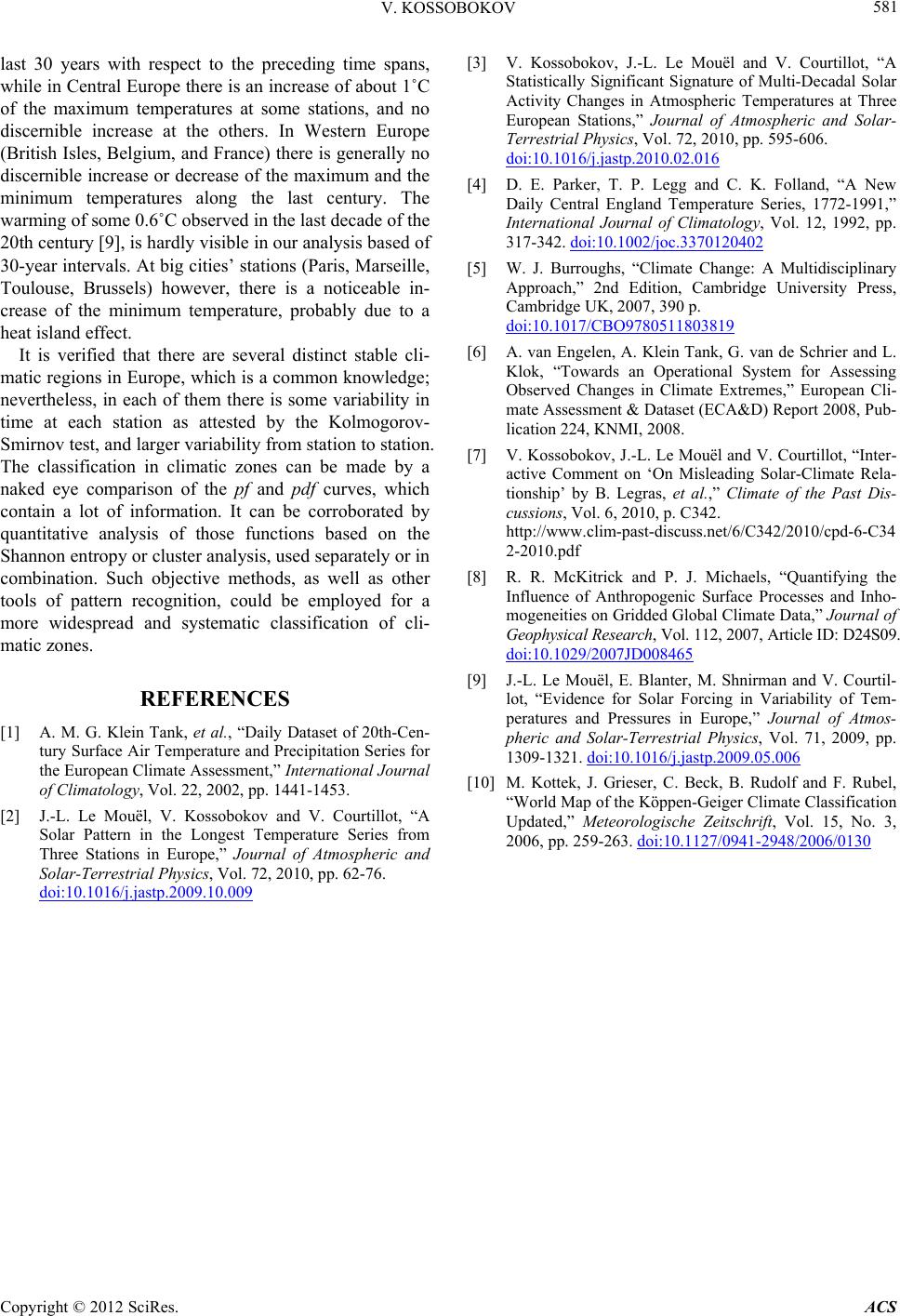

V. KOSSOBOKOV 581
last 30 years with respect to the preceding time spans,
while in Central Europe there is an increase of about 1˚C
of the maximum temperatures at some stations, and no
discernible increase at the others. In Western Europe
(British Isles, Belgium, and France) there is generally no
discernible increase or decrease of the maximum and the
minimum temperatures along the last century. The
warming of some 0.6˚C observed in the last decade of the
20th century [9], is hardly visible in our analysis based of
30-year intervals. At big cities’ stations (Paris, Marseille,
Toulouse, Brussels) however, there is a noticeable in-
crease of the minimum temperature, probably due to a
heat island effect.
It is verified that there are several distinct stable cli-
matic regions in Europe, which is a common knowledge;
nevertheless, in each of them there is some variability in
time at each station as attested by the Kolmogorov-
Smirnov test, and larger variability from station to station.
The classification in climatic zones can be made by a
naked eye comparison of the pf and pdf curves, which
contain a lot of information. It can be corroborated by
quantitative analysis of those functions based on the
Shannon entropy or cluster analysis, used separately or in
combination. Such objective methods, as well as other
tools of pattern recognition, could be employed for a
more widespread and systematic classification of cli-
matic zones.
REFERENCES
[1] A. M. G. Klein Tank, et al., “Daily Dataset of 20th-Cen-
tury Surface Air Temperature and Precipitation Series for
the European Climate Assessment,” International Journal
of Climatology, Vol. 22, 2002, pp. 1441-1453.
[2] J.-L. Le Mouël, V. Kossobokov and V. Courtillot, “A
Solar Pattern in the Longest Temperature Series from
Three Stations in Europe,” Journal of Atmospheric and
Solar-Terrestrial Physics, Vol. 72, 2010, pp. 62-76.
doi:10.1016/j.jastp.2009.10.009
[3] V. Kossobokov, J.-L. Le Mouël and V. Courtillot, “A
Statistically Significant Signature of Multi-Decadal Solar
Activity Changes in Atmospheric Temperatures at Three
European Stations,” Journal of Atmospheric and Solar-
Terrestrial Physics, Vol. 72, 2010, pp. 595-606.
doi:10.1016/j.jastp.2010.02.016
[4] D. E. Parker, T. P. Legg and C. K. Folland, “A New
Daily Central England Temperature Series, 1772-1991,”
International Journal of Climatology, Vol. 12, 1992, pp.
317-342. doi:10.1002/joc.3370120402
[5] W. J. Burroughs, “Climate Change: A Multidisciplinary
Approach,” 2nd Edition, Cambridge University Press,
Cambridge UK, 2007, 390 p.
doi:10.1017/CBO9780511803819
[6] A. van Engelen, A. Klein Tank, G. van de Schrier and L.
Klok, “Towards an Operational System for Assessing
Observed Changes in Climate Extremes,” European Cli-
mate Assessment & Dataset (ECA&D) Report 2008, Pub-
lication 224, KNMI, 2008.
[7] V. Kossobokov, J.-L. Le Mouël and V. Courtillot, “Inter-
active Comment on ‘On Misleading Solar-Climate Rela-
tionship’ by B. Legras, et al.,” Climate of the Past Dis-
cussions, Vol. 6, 2010, p. C342.
http://www.clim-past-discuss.net/6/C342/2010/cpd-6-C34
2-2010.pdf
[8] R. R. McKitrick and P. J. Michaels, “Quantifying the
Influence of Anthropogenic Surface Processes and Inho-
mogeneities on Gridded Global Climate Data,” Journal of
Geophysical Research, Vol. 112, 2007, Article ID: D24S09.
doi:10.1029/2007JD008465
[9] J.-L. Le Mouël, E. Blanter, M. Shnirman and V. Courtil-
lot, “Evidence for Solar Forcing in Variability of Tem-
peratures and Pressures in Europe,” Journal of Atmos-
pheric and Solar-Terrestrial Physics, Vol. 71, 2009, pp.
1309-1321. doi:10.1016/j.jastp.2009.05.006
[10] M. Kottek, J. Grieser, C. Beck, B. Rudolf and F. Rubel,
“World Map of the Köppen-Geiger Climate Classification
Updated,” Meteorologische Zeitschrift, Vol. 15, No. 3,
2006, pp. 259-263. doi:10.1127/0941-2948/2006/0130