Atmospheric and Climate Sciences, 2012, 2, 538-545
http://dx.doi.org/10.4236/acs.2012.24049 Published Online October 2012 (http://www.SciRP.org/journal/acs)
Communicating the Probabilities of Extreme Surface
Temperatur e Outcomes
Nathan Rive, Gunnar Myhre*
Center for International Climate and Environmental Research—Oslo (CICERO), Oslo, Norway
Received April 1, 2012; revised May 31, 2012; accepted June 10, 2012
ABSTRACT
The magnitude of the future global warming is uncertain, but the possible dramatic changes associated with high tem-
peratures have seen rising attention in the literature. Projections of temperature change in the literature are often pre-
sented in probabilistic terms and typically highlight the most likely ranges of future temperature under assumed emis-
sion scenarios. However, focusing on these high probability outcomes of global warming omits important information
related to the threats of low-probability but high-impact outcomes under more extreme change. As such, we argue that
the literature should place more emphasis on communicating the probabilities of extreme temperature change, in a way
that is accessible to policymakers and the general public. The damage associated with climate change is likely to be
non-linear with temperature, and thus extreme temperature changes may pose a larger risk than the most likely out-
comes. We use a simple climate model to explore the probabilities of high surface temperature under business as usual
emissions scenarios, given current knowledge of the climate system. In a business as usual scenario (A1FI) we find the
probability of “likely” warming (central 66%) to be approximately 4.4˚C - 6.9˚C in 2100 (above 1900 levels). However,
we find extreme (>7˚C) warming to embody a notable portion of damage risk compared to this likely range.
Keywords: Risk; Communication of Climate Change; Probability
1. Introduction
1.1. Background
While the potential damages are the ultimate concern,
among policymakers, academics, and the general public,
discussion on climate change is typically framed in terms
of rising global mean surface temperature. This is be-
cause temperature is a key indicator of changes to the
climate and it is familiar the general public. This is seen,
most notably, in the warming limit of 2˚C supported by
the European Union [1] and recognized by the Copenha-
gen Accord [2]. As such, strategies for responding to the
climate change are informed in part by projections of
temperature change in the coming century. However, the
knowledge of the climate system is incomplete and faces
compounded uncertainties [3], and as such these projec-
tions usually take a probabilistic format, indicating the
different likelihoods of particular temperature outcomes.
In many cases, such projections are developed via
Monte Carlo-style experiments in simple climate models,
capturing the uncertainty of key climate parameters such
as climate sensitivity, aerosol forcing, ocean heat diffu-
sivity and their impact on temperature change. Emissions
scenarios are run in the model over many iterations with
different combinations of these parameters. The particu-
lar parameter combinations are limited to those which
successfully replicate historical climate change. The re-
sulting set of temperature projections across all these
iterations is then used to construct the probability density
function (PDF) of temperature outcomes over time. A
number of studies have generated PDFs of future global
mean temperature change (and other outcomes) under
alternative business as usual [4,5] and mitigation [6] emis-
sion scenarios.
The central (most probable) temperature outcomes of
such projections are typically the focus in the literature.
Most notably, the IPCC Fourth Assessment Report (AR4)
Summary for Policymakers, presents a range of 1.1˚C -
6.4˚C for “likely” warming to 2100 across several busi-
ness as usual scenarios, where “likely” refers to the cen-
tral 66% probability range [3]. Associated figures for
these projections (e.g. Figure SPM.5 and 10.4 in AR4)
also only show the mean values and ±1 standard devia-
tion (σ) ranges. This may be for a number of reasons: a
tendency to focus on what is known best, and/or the use
of specific temperature targets to guide emissions reduc-
tions. Extreme temperature outcomes, which may have
very low likelihood, are often not presented.
*Corresponding author.
C
opyright © 2012 SciRes. ACS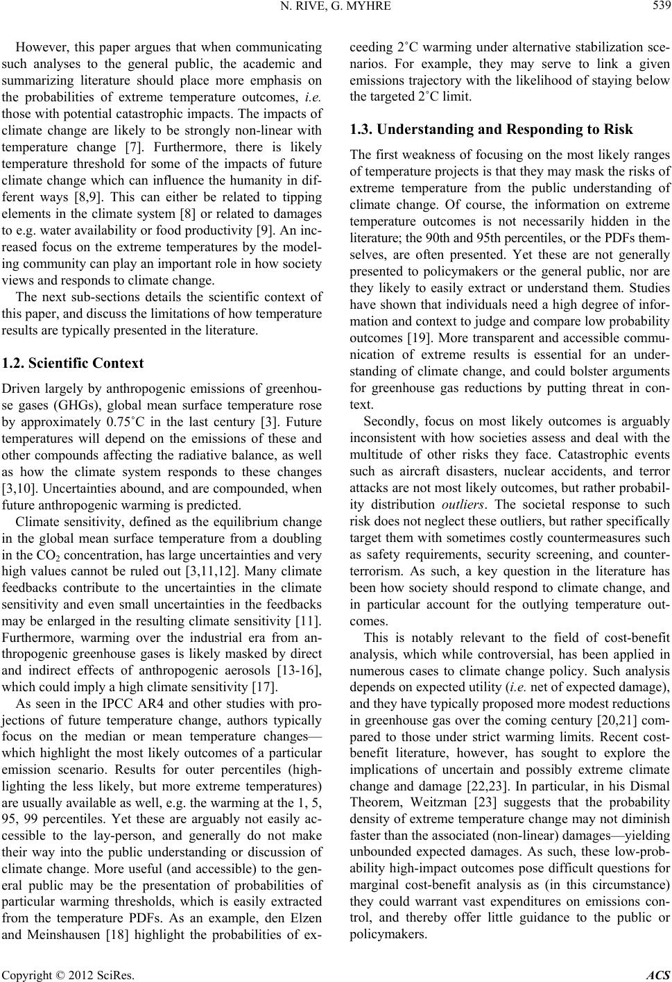

N. RIVE, G. MYHRE 539
However, this paper argues that when communicating
such analyses to the general public, the academic and
summarizing literature should place more emphasis on
the probabilities of extreme temperature outcomes, i.e.
those with potential catastrophic impacts. The impacts of
climate change are likely to be strongly non-linear with
temperature change [7]. Furthermore, there is likely
temperature threshold for some of the impacts of future
climate change which can influence the humanity in dif-
ferent ways [8,9]. This can either be related to tipping
elements in the climate system [8] or related to damages
to e.g. water availability or food productivity [9]. An inc-
reased focus on the extreme temperatures by the model-
ing community can play an important role in how society
views and responds to climate change.
The next sub-sections details the scientific context of
this paper, and discuss the limitations of how temperature
results are typically presented in the literature.
1.2. Scientific Context
Driven largely by anthropogenic emissions of greenhou-
se gases (GHGs), global mean surface temperature rose
by approximately 0.75˚C in the last century [3]. Future
temperatures will depend on the emissions of these and
other compounds affecting the radiative balance, as well
as how the climate system responds to these changes
[3,10]. Uncertainties abound, and are compounded, when
future anthropogenic warming is predicted.
Climate sensitivity, defined as the equilibrium change
in the global mean surface temperature from a doubling
in the CO2 concentration, has large uncertainties and very
high values cannot be ruled out [3,11,12]. Many climate
feedbacks contribute to the uncertainties in the climate
sensitivity and even small uncertainties in the feedbacks
may be enlarged in the resulting climate sensitivity [11].
Furthermore, warming over the industrial era from an-
thropogenic greenhouse gases is likely masked by direct
and indirect effects of anthropogenic aerosols [13-16],
which could imply a high climate sensitivity [17].
As seen in the IPCC AR4 and other studies with pro-
jections of future temperature change, authors typically
focus on the median or mean temperature changes—
which highlight the most likely outcomes of a particular
emission scenario. Results for outer percentiles (high-
lighting the less likely, but more extreme temperatures)
are usually available as well, e.g. the warming at the 1, 5,
95, 99 percentiles. Yet these are arguably not easily ac-
cessible to the lay-person, and generally do not make
their way into the public understanding or discussion of
climate change. More useful (and accessible) to the gen-
eral public may be the presentation of probabilities of
particular warming thresholds, which is easily extracted
from the temperature PDFs. As an example, den Elzen
and Meinshausen [18] highlight the probabilities of ex-
ceeding 2˚C warming under alternative stabilization sce-
narios. For example, they may serve to link a given
emissions trajectory with the likelihood of staying below
the targeted 2˚C limit.
1.3. Understanding and Responding to Risk
The first weakness of focusing on the most likely ranges
of temperature projects is that they may mask the risks of
extreme temperature from the public understanding of
climate change. Of course, the information on extreme
temperature outcomes is not necessarily hidden in the
literature; the 90th and 95th percentiles, or the PDFs them-
selves, are often presented. Yet these are not generally
presented to policymakers or the general public, nor are
they likely to easily extract or understand them. Studies
have shown that individuals need a high degree of infor-
mation and context to judge and compare low probability
outcomes [19]. More transparent and accessible commu-
nication of extreme results is essential for an under-
standing of climate change, and could bolster arguments
for greenhouse gas reductions by putting threat in con-
text.
Secondly, focus on most likely outcomes is arguably
inconsistent with how societies assess and deal with the
multitude of other risks they face. Catastrophic events
such as aircraft disasters, nuclear accidents, and terror
attacks are not most likely outcomes, but rather probabil-
ity distribution outliers. The societal response to such
risk does not neglect these outliers, but rather specifically
target them with sometimes costly countermeasures such
as safety requirements, security screening, and counter-
terrorism. As such, a key question in the literature has
been how society should respond to climate change, and
in particular account for the outlying temperature out-
comes.
This is notably relevant to the field of cost-benefit
analysis, which while controversial, has been applied in
numerous cases to climate change policy. Such analysis
depends on expected utility (i.e. net of expected damage),
and they have typically proposed more modest reductions
in greenhouse gas over the coming century [20,21] com-
pared to those under strict warming limits. Recent cost-
benefit literature, however, has sought to explore the
implications of uncertain and possibly extreme climate
change and damage [22,23]. In particular, in his Dismal
Theorem, Weitzman [23] suggests that the probability
density of extreme temperature change may not diminish
faster than the associated (non-linear) damages—yielding
unbounded expected damages. As such, these low-prob-
ability high-impact outcomes pose difficult questions for
marginal cost-benefit analysis as (in this circumstance)
they could warrant vast expenditures on emissions con-
trol, and thereby offer little guidance to the public or
policymakers.

N. RIVE, G. MYHRE
540
Furthermore, if society’s approach to climate policy
takes the form of hedging, this would require knowledge
of both the likely and extreme temperature probabilities.
A number of financial instruments are already in use (e.g.
credit default swaps, option contracts) to hedge against
loss or volatility, and additional instruments may be de-
veloped to insure against climate damages if particular
thresholds are exceeded [24]. Alternatively, climate
change hedging may take the form of emissions reduc-
tions targeted specifically at reducing the possibilities of
reaching key (potentially catastrophic) warming thresh-
olds in future [25], or ensuring future climate targets re-
main within reach [26].
1.4. Communicating Extreme Temperatures and
Risks
Given its importance to society’s understanding and re-
sponse to climate change, how, then, can the probabilities
of extreme temperature change be calculated and com-
municated by researchers? There is, of course, no one
correct answer. Instead, we are advocating “good prac-
tice” among climate modelers: presenting both the likely
and more extreme temperature outcomes of model pro-
jections, and seeking to do so in a way that is transparent
and accessible to general public and policymakers. Sev-
eral examples are discussed below, but this list is by no
means exhaustive.
A useful means of presenting extreme warming prob-
abilities is to focus on the probabilities of exceeding key
warming thresholds (e.g. the 2˚C limit). Anchoring the
results to particular temperature levels is arguably more
accessible to the layman than focusing on the probabili-
ties themselves (e.g. the top decile warming range), as
such temperatures can form the basis of particular cli-
mate goals or be associated with particular climate im-
pacts to the environment and economy. This could in-
clude risks of species extinction, coral bleaching, reduced
agricultural productivity under 2˚C - 3˚C warming [27,
Figure SPM.2]. This does not require the development of
new methodologies per se, and in principle such a per-
spective could be applied in most of the existing prob-
abilistic studies found in the literature.
2. Illustrative Modeling Exercise
As a means of supporting the above arguments, a model-
ing exercise is undertaken here to illustrate the probabili-
ties of large temperature changes in 2050 and 2100 under
alternative business as usual scenarios—the IPCC SRES
A1B, A1FI, and A2 marker scenarios [28]. These sce-
narios represent alternative emissions trajectories that are
unconstrained by climate policy under differing socio-ec-
onomic and technological trends. The emissions scenar-
ios are run in a simple climate model (SCM), in a
“What’s the worst that could happen?” examination of
unabated greenhouse gas emissions growth and potential
temperature outcomes of that growth [29], and in par-
ticular the probability distribution of the temperature
outcomes. The A1FI is the most “pessimistic” of the sce-
narios, with the highest cumulative emissions to 2100,
although it appears to best represent recent global emis-
sions trends [30].
In line with the “good practice” highlighted above,
alongside the most likely temperature outcome of these
scenarios we focus on two aspects of the more extreme
potential temperature changes: 1) the probabilities of
exceeding key warming thresholds, and 2) the risks asso-
ciated with extreme warming. While the methodologies
are largely line with existing techniques found in the lit-
erature, our focus on the high temperature results is
novel.
With regards to temperature thresholds, we explore the
probabilities of exceeding 2˚C, 2.5˚C, and 3˚C warming
(above 1900 levels) in 2050, and 5˚C, 6˚C, and 7˚C in
2100. The results are shown for various temperature
thresholds since different temperature changes may be
responsible for different impacts [27, Figure SPM.2].
Because these temperature changes are expected to yield
damages to the economy and environment, they can be
presented in terms of the risks that they effectively pose.
In particular, we can compare the risks posed by the
more extreme temperature outcomes (which may be less
likely, but result in large damages) to the risks posed by
the more moderate temperature outcomes (which may be
more likely, but with lesser damages). In this exercise we
do this by comparing each ranges’ contribution (C) to the
overall expected damages. This contribution is a simple
representation of risk, and is defined as:
 

2
1
12
()d
,
()d
t
tpTDT T
Ct t
pTDT T





 (1)
ΔT represents global mean surface temperature change,
assuming some future emissions trajectory and time pe-
riod. The variables p(ΔT) and D(ΔT) represent the asso-
ciated probability density and climate impact damage; t1
and t2 are the temperature ranges of concern (e.g. ex-
treme or most likely ranges).
The CICERO Simple Climate Model (SCM) is em-
ployed [31], used previously in several studies [32,33].
This model simulates global mean temperature change by
an energy-balance climate/up-welling diffusion ocean
model developed by Schlesinger et al. [34]. Climate sen-
sitivity and parameters which control the uptake of heat
by the oceans, are set exogenously, which govern the
climate response [35]. Historical emissions are taken
from publicly available databases [36,37]. Global mean
concentrations are calculated from emissions data and

N. RIVE, G. MYHRE 541
radiative forcing is calculated using concentration-forc-
ing relations from IPCC AR4 [13]. CO2 concentrations
are calculated using a scheme based on Joos et al. [38].
Where data is available, historical volcanic and solar
forcings are included. The model has recently been used
in another study where the climate sensitivity has been
derived the historical temperature record over last cen-
tury in a Bayesian framework [39].
Two approaches are adopted to calculate the probabili-
ties of surface temperatures changes. The aim is to mirror
their parallel use in the literature, and demonstrate how
methodological differences can impact the estimated
probabilities of extreme outcomes. The first approach
(labeled as “Feasible”) employs a Monte Carlo experi-
ment, running the scenarios multiple times under alterna-
tive model parameter assumptions, and constraining the
results by historical warming observations. Alternative
values of both climate sensitivity and aerosol forcing are
sampled from assumed prior probability distributions, in
a similar vein to other studies in the literature [4,17,40].
Latin Hypercube Sampling (LHS) is used with a sam-
ple size of 15,000. Prior probabilities for each parameter
are broken into equal probability segments, with each
segment randomly sampled only once. Values for indi-
rect sulphate forcing (uniform distribution) and direct
aerosol forcing (normal distribution) priors are taken
from AR4 (Table 2.12 in Chapter 2). The prior for cli-
mate sensitivity is assumed to take a Cauchy distribution
based (in part) on earlier expert opinion [41]1. See Table
1 below for the listing of these assumptions. Historical El
Nino-Southern Oscillation (ENSO), solar forcing, and
volcanic eruptions are accounted for. Each model run is
weighted by its replication of historical (1851-2005)
global mean surface temperature observations [42], as-
suming a first-order autoregressive model and normally
distributed error [43,44]. This weighting is then applied
to these parameter combinations and the associated tem-
perature projections via weighted kernel density estima-
tion, to generate posterior probability distributions of
these key climate parameters and temperature change
outcomes. The results of this approach (both temperature
outcomes and risks) are presented in the next section.
The second approach (labeled as “Best Estimate”)
treats the uncertainties of aerosol and climate sensitivity
separately. While it is not as comprehensive as the Feasi-
ble approach, it is seen elsewhere in the literature [18,33].
The model is only run using most likely values for aero-
sol forcing; for consistency these are taken from poste-
rior PDFs developed under the Feasible approach. The
probabilities of exceeding each threshold are calculated
via an “nverse lookup” of the posterior PDF of climate
sensitivity (also developed under the Feasible approach).
Specifically, the model is run (with best estimate aerosol
forcings) iteratively to find the equilibrium climate sensi-
tivity levels that yield each respective temperature
threshold level. For example, it is found that a climate
sensitivity of 3.0˚C will yield 2˚C warming (above 1900
levels) in 2050 under the A1B scenario. The cumulative
probability (and thus the probability of exceedance) of
this climate sensitivity level is then looked up on the
posterior PDF. These Best Estimate model results are
also presented and discussed in the next section.
3. Analysis of Modeling Results
3.1. Temperature Changes
Figure 1 presents probabilistic temperature change over
the period 2000-2100 for the SRES A1FI scenario under
the Best Estimate and Feasible approaches. The central
66% (likely) probability range and median warming in
the A1FI scenario are approximately 4.4˚C - 6.9˚C and
5.6˚C (above 1900 levels) respectively under both ap-
proaches. However, the central 90% range is notably
wider under the Best Estimate approach. This is because
it allows for combinations of high climate sensitivity and
weak aerosol forcing (and vice versa) that would be re-
jected (i.e. given a low weighting) in the Feasible appro-
ach, as they would poorly replicate historical warming.
3.2. Probabilities of Threshold Exceedance
The probabilities of exceeding key temperature thresh-
olds in 2050 and 2100 under the SRES scenarios is pre-
sented in Figure 2. The first striking result is that 2˚C, a
key threshold for the European Union and Copenhagen
Accord, is reached with more than 55% probability in all
these three scenarios in 2050. Under A1FI, the probabil-
ity is approximately 90%. Concerns have already been
raised over the adequacy of current commitments seeking
to limit warming below 2˚C [45].
For more extreme temperature levels in 2100, the re-
sults may be equally worrying. The probabilities of
reaching 5˚C warming by 2100 are substantial—between
Table 1. Prior probability distributions for model param-
eters in Feasible approach. Forcing taken to be change in
forcing between 1 750 -2 005 . C li mat e sensitivit y is taken to be
˚C per doubling of CO2 concentration at equilibrium.
Model ParameterUnitsPrior
Distribution
Distribution
Parameters Source
SO4 Forcing (direct)W/m2Normal μ: –0.4, σ: 0.12[13]
SO4 Cloud EffectW/m2Uniform range:
–1.9 to –0.22[13]
Black Carbon
Forcing (direct) W/m2Normal μ: 0.2, σ: 0.09[13]
Organic Carbon
Forcing (direct) W/m2Normal μ: –0.05, σ: 0.03[13]
Climate Sensitivity˚C Cauchy loc: 2, scale: 3.5[41]
1Truncated at 0˚C and 20˚C per doubling of CO2 concentration.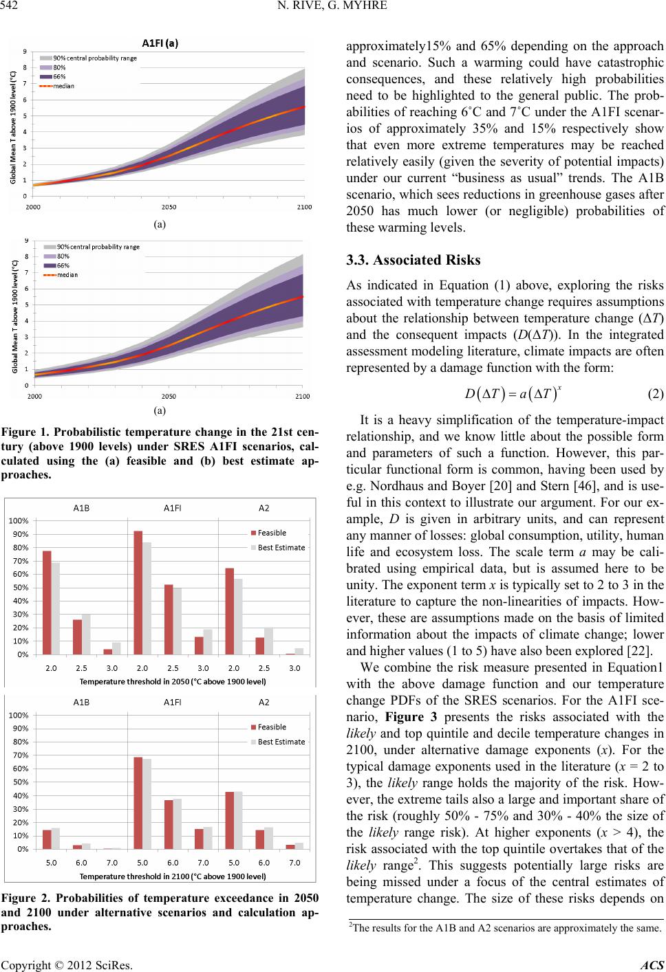

N. RIVE, G. MYHRE
542
(a)
(a)
Figure 1. Probabilistic temperature change in the 21st cen-
tury (above 1900 levels) under SRES A1FI scenarios, cal-
culated using the (a) feasible and (b) best estimate ap-
proaches.
Figure 2. Probabilities of temperature exceedance in 2050
and 2100 under alternative scenarios and calculation ap-
proaches.
approximately15% and 65% depending on the approach
and scenario. Such a warming could have catastrophic
consequences, and these relatively high probabilities
need to be highlighted to the general public. The prob-
abilities of reaching 6˚C and 7˚C under the A1FI scenar-
ios of approximately 35% and 15% respectively show
that even more extreme temperatures may be reached
relatively easily (given the severity of potential impacts)
under our current “business as usual” trends. The A1B
scenario, which sees reductions in greenhouse gases after
2050 has much lower (or negligible) probabilities of
these warming levels.
3.3. Associated Risks
As indicated in Equation (1) above, exploring the risks
associated with temperature change requires assumptions
about the relationship between temperature change (ΔT)
and the consequent impacts (D(ΔT)). In the integrated
assessment modeling literature, climate impacts are often
represented by a damage function with the form:
 
x
DT aT (2)
It is a heavy simplification of the temperature-impact
relationship, and we know little about the possible form
and parameters of such a function. However, this par-
ticular functional form is common, having been used by
e.g. Nordhaus and Boyer [20] and Stern [46], and is use-
ful in this context to illustrate our argument. For our ex-
ample, D is given in arbitrary units, and can represent
any manner of losses: global consumption, utility, human
life and ecosystem loss. The scale term a may be cali-
brated using empirical data, but is assumed here to be
unity. The exponent term x is typically set to 2 to 3 in the
literature to capture the non-linearities of impacts. How-
ever, these are assumptions made on the basis of limited
information about the impacts of climate change; lower
and higher values (1 to 5) have also been explored [22].
We combine the risk measure presented in Equation1
with the above damage function and our temperature
change PDFs of the SRES scenarios. For the A1FI sce-
nario, Figure 3 presents the risks associated with the
likely and top quintile and decile temperature changes in
2100, under alternative damage exponents (x). For the
typical damage exponents used in the literature (x = 2 to
3), the likely range holds the majority of the risk. How-
ever, the extreme tails also a large and important share of
the risk (roughly 50% - 75% and 30% - 40% the size of
the likely range risk). At higher exponents (x > 4), the
risk associated with the top quintile overtakes that of the
likely range2. This suggests potentially large risks are
being missed under a focus of the central estimates of
temperature change. The size of these risks depends on
2The results for the A1B and A2 scenarios are approximately the same.

N. RIVE, G. MYHRE 543
Figure 3. Risk (measured as the contribution to expected
damage, see Equation (1) from likely and “extreme” ranges
of temperature change in 2100 under the A1FI scenario.
Damage function is taken from Equation (2) above.
the shape of the temperature PDF and the damage func-
tion assumptions. If our temperature PDF had a “fatter”
right-hand tail (i.e. higher likelihood of extreme tem-
perature change), or if the damage function accounted for
larger damages at higher temperature (e.g. irreversible
singular events), the risks of extreme temperatures com-
pared to the most likely outcomes would be even larger.
4. Caveats and Challenges
It goes without saying that we have not presented an ex-
haustive picture of how extreme temperatures should be
discussed in the literature. A key hurdle remains with
respect to how they can be calculated. The paradox, of
course, is that we are advocating an increased focus on
outcomes of which we are least certain. Probabilistic
results will depend heavily on the applied model, meth-
odologies and assumptions, and subjectivities. The hope,
is that over time the literature will have developed a
range of the probabilities of extreme outcomes, in the
same way that “likely” ranges have been presented (e.g.
in the IPCC AR4).
Neither have we offered a solution to how policymak-
ers would then use such information to formulate a re-
sponse. Individuals (and societies) are often poor evalua-
tors of risk, particularly with respect to low-probability
high-impact outcomes [19], and policy responses to
threats are rarely consistent. One example of such an
inconsistency is the “One Percent Doctrine” applied by
the Bush Administration towards terrorism, by which a
1% chance of a low-probability high-impact event (e.g.
acquisition of nuclear bomb by al-Qaeda) was to be acted
upon as if it were certain to occur [47]. It goes without
saying that the Administration’s climate change policy
did not feature the same approach. Furthermore, along-
side to the damage risks, we should in principle consider
the mitigation risks; mitigation may turn out to be more
expensive or disruptive than expected. Or there may be a
policy overreaction with excessive (costly) mitigation.
Such “action bias” is highly relevant to climate change
given potentially emotional responses to what may be at
stake [48].
5. Conclusions
In this paper, we argue that for the general public’s (and
policymakers’) consideration of climate change, the
probability of extreme warming is key information that is
often missing in the public debate. Extreme temperature
change outcomes, even if they have low likelihood of
occurring, pose a large risk compared to the likely ranges,
which needs to be highlighted. However, the likelihood
of these extremes has tended to be under-represented in
the modeling literature.
The method outlined here can be improved by either
physical parameters important for the simple climate
model [49] or improved work on the radiative forcing
time series [50]. However, the results outlined here can
also be derived from a larger set of Atmospheric Ocean
General Circulation Models (AOGCMs) or ensemble
simulations in one AOGCM [12]. Thus, the main empha-
sis of this study on extreme temperature outcomes and
associated risks can be derived by various methods and
model complexities.
The extreme temperature probabilities can play a key
role in shaping public attitudes to climate change and the
development of responses. Knowledge of these extremes
may directly inform the development of climate change
mitigation policy, including those based on cost-benefit
analysis and hedging strategies. We advocate for “good
practice” among climate modelers to better communicate
the probabilities of extreme outcomes alongside the most
likely temperature ranges.
The paper supports these arguments using an illustra-
tive modeling exercise to highlight the probabilities of
exceeding key temperature thresholds by 2100. Under
the SRES A1FI scenario in 2100, there is a notable prob-
ability (>60%) of exceeding 5˚C, whereas the central
66% probability range is approximately 4.4˚C - 6.9˚C.
Likewise the probability to exceed 6˚C in this scenario is
35% - 40% and more than 15% to exceed 7˚C. What the
results suggest is the surprising ease by which a business
as usual can lead to extreme temperatures in future, a
point that has been under-reported in the summarizing
and scientific literature so far.
6. Acknowledgements
The authors thank Katsumasa Tanaka for comments and

N. RIVE, G. MYHRE
544
collaboration on the modeling methodology. This work
was funded in part by the Norwegian Research Council
(NFR) Strategic Institute Program.
REFERENCES
[1] European Commission, “Decision of the European Par-
liament and of the Council on the Effort of Member
States to Reduce Their Greenhouse Gas Emissions to
Meet the Community’s Greenhouse Gas Emission Reduc-
tion Commitments up to 2020,” 2008.
[2] UNFCCC, “Draft decision-/CP.15: Copenhagen Accord,”
Conference of Parties, Copenhagen, 2009.
[3] IPCC, “The Physical Science Basis. Contribution of
Working Group I to the Fourth Assessment Report of the
Intergovernmental Panel on Climate Change,” Cambridge
University Press, Cambridge, 2007.
[4] R. Knutti, T. F. Stocker, F. Joos and G. K. Plattner,
“Probabilistic Climate Change Projections Using Neural
Networks,” Climate Dynamics, Vol. 21, No. 3-4, 2003, pp.
257-272. doi:10.1007/s00382-003-0345-1
[5] T. M. L. Wigley and S. C. B. Raper, “Interpretation of
High Projections for Global-Mean Warming,” Science,
Vol. 293, No. 5529, 2001, pp. 451-454.
doi:10.1126/science.1061604
[6] M. Meinshausen, et al., “Greenhouse-Gas Emission Tar-
gets for Limiting Global Warming to 2 Degrees C,” Na-
ture, Vol. 458, No. 7242, 2009, pp. 1158-1162.
doi:10.1038/nature08017
[7] R. S. J. Tol, “The Economic Effects of Climate Change,”
Journal of Economic Perspectives, Vol. 23, No. 2, 2009,
pp. 29-51. doi:10.1257/jep.23.2.29
[8] T. M. Lenton, et al., “Tipping Elements in the Earth’s
Climate System,” Proceedings of the National Academy
of Sciences of the United States of America, Vol. 105, No.
6, 2008, pp. 1786-1793. doi:10.1073/pnas.0705414105
[9] M. L. Parry, O. F. Canziani, J. P. Palutikof and Co-Au-
thors, “Technical Summary. Climate Change 2007: Im-
pacts, Adaptation and Vulnerability,” In: M. L. Parry, et
al., Eds., Contribution of Working Group II to the Fourth
Assessment Report of the Intergovernmental Panel on
Climate Change, Cambridge University Press, Cambridge,
2007.
[10] J. Hansen, et al., “Dangerous Human-Made Interference
with Climate: A GISS Modele Study,” Atmospheric Che-
mistry and Physics, Vol. 7, No. 9, 2007, pp. 2287-2312.
doi:10.5194/acp-7-2287-2007
[11] G. H. Roe and M. B. Baker, “Why Is Climate Sensitivity
So Unpredictable?” Science, Vol. 318, No. 5850, 2007,
pp. 629-632. doi:10.1126/science.1144735
[12] D. A. Stainforth, et al., “Uncertainty in Predictions of the
Climate Response to Rising Levels of Greenhouse Gases,”
Nature, Vol. 433, No. 7024, 2005, pp. 403-406.
doi:10.1038/nature03301
[13] P. Forster, et al., “Changes in Atmospheric Constituents
and in Radiative Forcing, in Climate Change 2007: The
Physical Science Basis,” In: S. Solomon, et al., Eds.,
Contribution of Working Group I to the Fourth Assess-
ment Report of the Intergovernmental Panel on Climate
Change, Cambridge University Press, Cambridge, 2007.
[14] J. Hansen, et al., “Earth’s Energy Imbalance: Confirma-
tion and Implications,” Science, Vol. 308, No. 5727, 2005,
pp. 1431-1435. doi:10.1126/science.1110252
[15] Y. J. Kaufman, D. Tanre and O. Boucher, “A Satellite
View of Aerosols in the Climate System,” Nature, Vol.
419, No. 6903, 2002, pp. 215-223.
doi:10.1038/nature01091
[16] G. Myhre, “Consistency between Satellite-Derived and
Modeled Estimates of the Direct Aerosol Effect,” Science,
Vol. 325, No. 5937, 2009, pp. 187-190.
doi:10.1126/science.1174461
[17] M. O. Andreae, C. D. Jones and P. M. Cox, “Strong Pre-
sent-Day Aerosol Cooling Implies a Hot Future,” Nature,
Vol. 435, No. 7046, 2005, pp. 1187-1190.
doi:10.1038/nature03671
[18] M. G. J. den Elzen and M. Meinshausen, “Multi-Gas
Emission Pathways for Meeting the EU 2˚C Climate
Target in Avoiding Dangerous Climate Change,” Cam-
bridge University Press, Cambridge, 2006.
[19] H. Kunreuther, N. Novemsky and D. Kahneman, “Mak-
ing Low Probabilities Useful,” Journal of Risk and Un-
certainty, Vol. 23, No. 2, 2001, pp. 103-120.
doi:10.1023/A:1011111601406
[20] W. D. Nordhaus and J. Boyer, “Warming the World:
Economic Models of Global Warming,” Cambridge Uni-
versity Press, Cambridge, 2000.
[21] R. S. J. Tol, “On the Optimal Control of Carbon Dioxide
Emissions: An Application of FUND,” Environmental
Modeling and Assessment, Vol. 2, No. 3, 1997, pp. 151-
163. doi:10.1023/A:1019017529030
[22] F. Ackerman, E. A. Stanton and R. Bueno, “Fat Tails,
Exponents, Extreme Uncertainty: Simulating Catastrophe
in DICE,” Ecological Economics, Vol. 69, No. 8, 2010,
pp. 1657-1665. doi:10.1016/j.ecolecon.2010.03.013
[23] M. L. Weitzman, “On Modeling and Interpreting the
Economics of Catastrophic Climate Change,” Review of
Economics and Statistics, Vol. 91, No. 1, 2009, pp. 1-19.
doi:10.1162/rest.91.1.1
[24] H. C. Kunreuther and E. O. Michel-Kerjan, “The Devel-
opment of New Catastrophe Risk Markets,” Annual Re-
view of Resource Economics, Vol. 1, 2009, pp. 119-137.
[25] M. L. Weitzman, “GHG Targets as Insurance agains
Catastrophic Climate Damages,” Harvard University,
Cambridge, 2009.
[26] G. Yohe, N. Andronova and M. Schlesinger, “Climate—
To Hedge or Not against an Uncertain Climate,” Science,
Vol. 306, No. 5695, 2004, pp. 416-417.
doi:10.1126/science.1101170
[27] IPCC, “Summary for Policymakers, in Climate Change
2007: Impacts, Adaptation and Vulnerability,” In: M. L.
Parry, et al., Eds., Contribution of Working Group II to
the 4th Assessment Report of the Intergovernmental Panel
on Climate Change, Cambridge University Press, Cam-
bridge, 2007, p. 16.
[28] N. Nakicenovic and R. Swart, “Special Report of Work-
ing Group III of the Intergovernmental Panel on Climate

N. RIVE, G. MYHRE
545
Change,” Cambridge Univeristy Press, Cambridge, 2000.
[29] S. Schneider, “The Worst-Case Scenario,” Nature, Vol.
458, No. 7242, 2009, pp. 1104-1105.
doi:10.1038/4581104a
[30] G. Myhre, K. Alterskjaer and D. Lowe, “A Fast Method
for Updating Global Fossil Fuel Carbon Dioxide Emis-
sions,” Environmental Research Letters, Vol. 4, No. 3,
2009, Article ID: 034012.
doi:10.1088/1748-9326/4/3/034012
[31] J. S. Fuglestvedt and T. Berntsen, “A Simple Model for
Scenario Studies of Changes in Global Climate: Version
1.0,” 1999.
[32] J. S. Fuglestvedt, et al., “Metrics of Climate Change:
Assessing Radiative Forcing and Emission Indices,” Cli-
matic Change, Vol. 58, No. 3, 2003, pp. 267-331.
doi:10.1023/A:1023905326842
[33] N. Rive, A. Torvanger, T. Berntsen and S. Kallbekken,
“To What Extent Can a Long-Term Temperature Target
Guide Near-Term Climate Change Commitments?” Cli-
matic Change, Vol. 82, No. 3-4, 2007, pp. 373-391.
doi:10.1007/s10584-006-9193-4
[34] M. Schlesinger, M. E. Jiang and R. J. Charlson, “Implica-
tion of Anthropogenic Atmospheric Sulphate for the Sen-
sitivity of the Climate System,” Proceedings of the In-
ternational Conference on Global Climate Change, New
York, 1992.
[35] D. Harvey, et al., “An Introduction to Simple Climate
Models Used in the IPCC Second Assessment Report,”
1997.
[36] European Commissionand Joint Research Centre, “Emis-
sion Database for Global Atmospheric Research (ED-
GAR), Release Version 4.0,” 2009.
[37] T. Boden, G. Marland and R. J. Andres, “National CO2
Emissions from Fossil-Fuel Burning, Cement Manufac-
ture, and Gas Flaring: 1751-2006,” 2009.
[38] F. Joos, et al., “An Efficient and Accurate Representation
of Complex Oceanic and Biospheric Models of Anthro-
pogenic Carbon Uptake,” Tellus Series B-Chemical and
Physical Meteorology, Vol. 48, No. 3, 1996, pp. 397-417.
doi:10.1034/j.1600-0889.1996.t01-2-00006.x
[39] M. Aldrin, et al., “Bayesian Estimation of Climate Sensi-
tivity Based on a Simple Climate Model Fitted to Obser-
vations of Hemispheric Temperatures and Global Ocean
Heat Content,” Environmetrics, Vol. 23, No. 3, 2012, pp.
253-271. doi:10.1002/env.2140
[40] A. P. Sokolov, et al., “Probabilistic Forecast for Twenty-
First-Century Climate Based on Uncertainties in Emis-
sions (without Policy) and Climate Parameters,” Journal
of Climate, Vol. 22, No. 19, 2009, pp. 5175-5204.
doi:10.1175/2009JCLI2863.1
[41] J. D. Annan and J. C. Hargreaves, “On the Generation
and Interpretation of Probabilistic Estimates of Climate
Sensitivity,” Climatic Change, Vol. 104, No. 3-4, 2011,
pp. 423-436. doi:10.1007/s10584-009-9715-y
[42] P. Brohan, J. J. Kennedy, I. Harris, S. F. B. Tett and P. D.
Jones, “Uncertainty Estimates in Regional and Global
Observed Temperature Changes: A New Data Set from
1850,” Journal of Geophysical Research-Atmospheres,
Vol. 111, No. D12, 2006, Article ID: D12106.
doi:10.1029/2005JD006548
[43] E. Kriegler, “Imprecise Probability Analysis for Inte-
grated Assessment of Climate Change,” Potsdam Univer-
sity, Potsdam, 2005.
[44] H. von Storch and F. W. Zwiers, “Statistical Analysis in
Climate Research,” Cambridge University Press, Cam-
bridge, 2002.
[45] J. Rogelj, et al., “Copenhagen Accord Pledges Are Pal-
try,” Nature, Vol. 464, No. 7292, 2010, pp. 1126-1128.
doi:10.1038/4641126a
[46] Stern, “The Economics of Climate Change: The Stern
Review,” 2006.
[47] R. Suskind, “The One Percent Doctrine: Deep Inside
America’s Pursuit of Its Enemies Since 9/11,” Simon &
Schuster, New York, 2006.
[48] C. R. Sustein and R. Zeckhauser, “Overreaction to Fear-
some Risks,” Environmental Resource Economics, in
Press.
[49] D. Olivie and N. Stuber, “Emulating AOGCM Results
Using Simple Climate Models,” Climate Dynamics, Vol.
35, No. 7-8, 2010, pp. 1257-1287.
doi:10.1007/s00382-009-0725-2
[50] R. B. Skeie, et al., “Anthropogenic Radiative Forcing
Time Series from Pre-Industrial Times until 2010,” At-
mospheric Chemistry and Physics, Vol. 11, No. 22, 2011,
pp. 11827-11857.
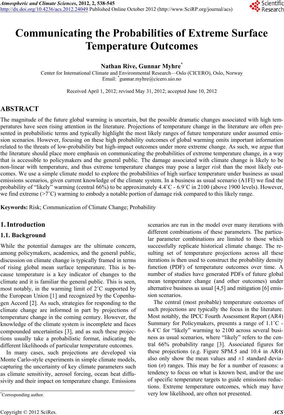