Atmospheric and Climate Sciences, 2012, 2, 492-500
http://dx.doi.org/10.4236/acs.2012.24043 Published Online October 2012 (http://www.SciRP.org/journal/acs)
Experimental and Parameterization Method for
Evaluation of Dry Deposition of S Compounds to
Natural Surfaces
Ranjit Kumar1, K. Maharaj Kumari2*
1Department of Applied Sciences, Technical College, Agra, India
2Department of Chemistry, Faculty of Science, Dayalbagh Educational Institute, Agra, India
Received March 10, 2012; revised April 15, 2012; accepted April 27, 2012
ABSTRACT
This paper deals with parameterization method based on meteorological parameters for calculation of dry deposition of
S compounds on natural surface (leaf of Cassia siamea) and direct measurement method. A scheme based on meteoro-
logical parameters has been evolved to calculate the dry deposition theoretically and a computer program has been de-
veloped. Experimentally dry deposition flux of S on leaf of Cassia siamea was measured by exposing the leaf surfaces
on non-dewy, non-foggy and non rainy days and washing the leaf surfaces with deionised water and samples were ana-
lyzed by Dionex Dx-500 Ion Chromatograph. Atmospheric concentration of SO2 was 3.54 ± 1.41 g·m–3 and particulate
was 2.72 ± 1.15 g·m–3. Theoretically obtained dry deposition velocity of SO2 and are 0.32 cm·s–1 and
0.75 cm·s–1, respectively. The calculated deposition of S as total sulphate (gaseous SO2 and particulate ) to Cassia
leaf was 2.05 ± 0.78 mg·m–2·d–1 and experimentally obtained dry deposition of S as sulphate was 1.07 ± 1.35
mg· m–2·d–1. The experimentally and theoretically obtained mean values for S as
2
4
SO 2
4

2
4
SO 
SO
2
4
SO

are comparable.
Keywords: Flux; Deposition Velocity; Parameterization; Sulphur; Gas and Particulate
1. Introduction
Atmospheric pollutants are deposited to ecosystems pri-
marily through wet deposition and dry deposition. Dry
deposition includes gases and particles. The primary
gases of major concern are nitric acid (HNO3), and sulfur
dioxide (SO2), while the primary particles are nitrate
(3) and sulfate (4
SO ) ions (Hanson and Lindberg,
1991 [1]). Sulphur is ubiquitous in nature and exists in
soil as organic compounds and as sulphur or sulphide, in
sea water as sulphate, in plants as sulphite, sulphide or
organic compound and in the atmosphere in gaseous and
solid states (Delmas and Servant, 1988 [2]). Sulphur
compounds have been considered as one of the potential
acidifying agents. Although much progress has been
made to control sulfur dioxide emissions, deposition of
sulfur (S) compounds continues to be a problem in Asia,
as a result, certain sensitive freshwater lakes and streams
continue to lose acid-neutralizing capacity (ANC) and
sensitive soils continue to be acidified. These acids result
from atmospheric oxidation of the sulfur dioxide (SO2)
released into the atmosphere during the smelting of ores
and from burning of fuels with the high sulfur content
and many other sources (Galloway et al., 1984 [3]).
NO 2

Dry deposition is one of the major mechanisms by
which air pollutants can be delivered to sensitive surfaces.
This process is governed by the concentration in air and
by turbulent transport processes in the boundary layer, by
the chemical and physical nature of the depositing spe-
cies and by the capability of the surface to capture or
absorb gases and particles (Hicks et al., 1987 [4]). Dry
deposition is usually characterized by deposition velocity
(Vd), which is defined as the flux (F) of the species (S) to
the surface divided by the concentration [S] at some ref-
erence height:
F
d
VS


The amount of the species deposited per unit area per
second in a geographical location, i.e., the flux, can be
calculated if the deposition velocity and the pollutant
concentration are known. The deposition velocity is also
frequently related to resistance (r):
d
1
VR 
*Corresponding author.
C
opyright © 2012 SciRes. ACS

R. KUMAR, K. M. KUMARI 493
By analogy to electrical systems, the resistance R can
be thought of as being comprised of several components
in dry deposition to ground are separated (Thom, 1975
[5]; Garland, 1977 [6]; Wesley and Hicks, 1977 [7];
Fowler, 1978 [8]): the aerodynamic resistance (Ra), the
quasilaminar resistance (Rb) and Canopy or surface re-
sistance (Rc). The inverse of the sum of the resistances
gives the deposition velocity,
d
V
abc
1
RRR
Dry deposition is much more difficult to estimate than
wet deposition. The estimation of dry deposition rates
requires information on the ambient concentrations of
pollutants, meteorological data, and information on land
use, vegetation, and surface conditions, all of which are
site-specific. Because of this site-specificity, it is difficult
to spatially extrapolate dry deposition data, as is often
done for wet deposition data.
A broad range of techniques has been used to measure
dry deposition (Businger, 1986 [9]). It can be divided
into two general categories: direct and indirect. Direct
method includes surrogate surfaces, natural surfaces,
chamber method, eddy correlation and eddy accumula-
tion methods for estimation of dry deposition. An indi-
rect method includes gradient method, inferential method
for determining dry deposition (Seinfeld and Pandis,
1998 [10]). Many dry deposition models (Acid Deposi-
tion and Oxidant Model, Regional Acid Deposition
Model, Dutch Empirical Acid Deposition Model) have
been developed during the past ten years and efforts con-
tinue to improve their capabilities (Wesley and Hicks,
2000 [11]). The dry deposition module in the Acid
Deposition and Oxidant Model (ADOM) was initially
developed in the early 1980s (Pleim et al., 1984 [12])
and has undergone testing and revisions (Padro and Ed-
wards, 1991 [13]; Padro, 1996 [14]). The Regional Acid
Deposition Model (RADM) has a dry deposition module
(Chang et al., 1987 [15]; Walcek et al., 1986 [16]), the
latest completed version of which was also described
(Wesley, 1989 [17]; Walmsley and Wesley, 1996 [18]).
Several models have been developed in Europe viz., the
Estimation of Deposition of Acidifying Components in
Europe (EDACS) and the Dutch Empirical Acid Deposi-
tion Model (DEADM) have been used with long-range
modules to map modeled deposition amounts for sulphur
and nitrogen compounds (Erisman and Draaijers, 1995
[19]). Parameterization methods have been developed
and tested extensively (Voldner et al., 1986 [20]; Hicks
et al., 1985 [21]; Meyers and Baldochhi, 1988 [22];
Wesley, 1989 [17]; Matt and Womack, 1989 [23]; Padro
et al., 1991 [24]; Stocker et al., 1993 [25]). In all the
studies assumptions and presumptions have been made.
All these study have limitations and need further im-
provements (Wesley and Hicks, 2000 [11]).
Direct measurement of dry deposition is expensive and
cumbersome in long-term measurements, so, an alternate
method was required to calculate the dry deposition. Dry
deposition can be determined by parameterization meth-
od by calculating the three resistances (Ra, Rb, and Rc)
governing dry deposition. In earlier reported studies de-
termination of Ra, Rb, and Rc together has not been made.
Hence, the present study was planned to determine aero-
dynamic resistance (Ra), quassilaminar resistance (Rb)
and surface resistance (Rc) using meteorological data and
to calculate the deposition flux and compare it with ex-
perimentally determined dry deposition flux to leaf of
Cassia (Cassia siamea) plant. As theoretical calculations
require numerous steps a computer program has been
developed. The present study is more accurate, realistic
and rigorous.
2. Methods and Materials
2.1. Theoretical Calculation
In the present study dry deposition velocity was calcu-
lated by simulating the different processes that govern
the dry deposition. The deposition velocity for gases is
based on
d
abc
1
VRRR  (1)
and that for particles on
ds
ababs
1
VV
RRRRV (2)




1
2
a4Ru




1
2
a9Ru



where,
Ra = aerodynamic resistance,
Rb = quassilaminar resistance,
Rc = surface resistance,
Vs = settling velocity
To calculate the Vd, the aerodynamic resistance (Ra),
quassilaminar resistance (Rb) and surface resistance (Rc)
were calculated by computing the values of meteoro-
logical data.
Aerodynamic Resistance
The aerodynamic resistance for both gases and particle
is calculated by
(3)
in neutral and stable stratification while in unstable con-
dition the equation is
(4)
where, u = mean wind speed and σ
 = standard deviation
of wind direction.
Quasilaminar Resistance
The quasilaminar resistances for gases and particles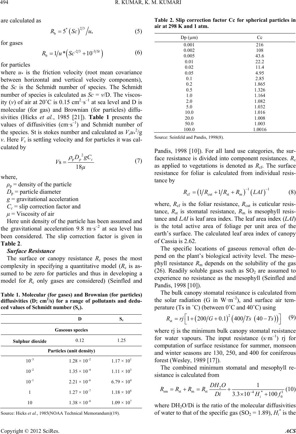

R. KUMAR, K. M. KUMARI
494
are calculated as

23
*
b
*
5RScu (5)
for gases

-2 3-3
10
St
Sc
b1*Ru (6)
for particles
where u* is the friction velocity (root mean covariance
between horizontal and vertical velocity components),
the Sc is the Schmidt number of species. The Schmidt
number of species is calculated as Sc = v/D. The viscos-
ity (v) of air at 20˚C is 0.15 cm2·s–1 at sea level and D is
molecular (for gas) and Brownian (for particles) diffu-
sivities (Hicks et al., 1985 [21]). Table 1 presents the
values of diffusivities (cm·s–1) and Schmidt number of
the species. St is stokes number and calculated as Vsu*2/g
v. Here Vs is settling velocity and for particles it was cal-
culated by
2
p
18
s
p
c
DgC
µ

V (7)
where,
ρp = density of the particle
Dp = particle diameter
g = gravitational acceleration
Cc = slip correction factor and
μ = Viscosity of air
Here unit density of the particle has been assumed and
the gravitational acceleration 9.8 m·s–2 at sea level has
been considered. The slip correction factor is given in
Table 2.
Surface Resistance
The surface or canopy resistance Rc poses the most
complexity in specifying a quantitative model (Rc is as-
sumed to be zero for particles and thus in developing a
model for Rc only gases are considered) (Seinfled and
Table 1. Molecular (for gases) and Brownian (for particles)
diffusivities (D; cm2/s) for a range of pollutants and dedu-
ced values of Schmidt number (Sc).
D Sc
Gaseous species
Sulphur dioxide 0.12 1.25
Particles (unit density)
10–3 1.28 × 10–2 1.17 × 101
10–2 1.35 × 10–4 1.11 × 103
10–1 2.21 × 10–6 6.79 × 104
1 1.27 × 10–7 1.18 × 106
10 1.38 × 10–8 1.09 × 107
Source: Hicks et al., 1985(NOAA Technical Memorandum)(19).
Table 2. Slip correction factor Cc for spherical particles in
air at 298 K and 1 atm.
Dp (µm) Cc
0.001
0.002
0.005
0.01
0.02
0.05
0.1
0.2
0.5
1.0
2.0
5.0
10.0
20.0
50.0
100.0
216
108
43.6
22.2
11.4
4.95
2.85
1.865
1.326
1.164
1.082
1.032
1.016
1.008
1.003
1.0016
Source: Seinfeld and Pandis, 1998(8).
Pandis, 1998 [10]). For all land use categories, the sur-
face resistance is divided into component resistances. Rc
as applied to vegetations is denoted as Rcf. The surface
resistance for foliar is calculated from individual resis-
tance by
 
11
cfcutst m
11RRRRLAI

 (8)
where, Rcf is the foliar resistance, Rcut is cuticular resis-
tance, Rst is stomatal resistance, Rm is mesophyll resis-
tance and LAI is leaf area index. The leaf area index (LAI)
is the total active area of foliage per unit area of the
earth’s surface. The calculated leaf area index of canopy
of Cassia is 2.62.
The specific locations of gaseous removal often de-
pend on the plant’s biological activity level. The meso-
phyll resistance Rm depends on the solubility of the gas
(26). Readily soluble gases such as SO2 are assumed to
experience no resistance as the mesophyll (Seinfled and
Pandis, 1998 [10]).
The bulk canopy stomatal resistance is calculated from
the solar radiation (G in W·m–2), and surface air tem-
perature (Ts in ˚C) (between 0˚C and 40˚C) using

 
2
st 12000.1400 40RrjGTs Ts (9)


 


where rj is the minimum bulk canopy stomatal resistance
for water vapours. The input resistance (s·m–1) rj for
computation of surface resistance for summer, monsoon
and winter seasons are 130, 250, and 400 for coniferous
forest (Wesley, 1989 [17]).
The combined minimum stomatal and mesophyll re-
sistance is calculated from
2
sm stm st4* 1
0
1
3.3 10100
i
DH O
RRRR
Di
H
f

  (10)
where DH2O/Di is the ratio of the molecular diffusivities
of water to that of the specific gas (SO2 = 1.89), Hi
* is the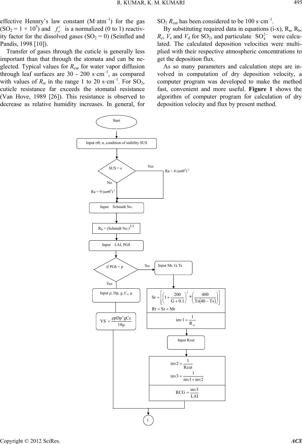

R. KUMAR, K. M. KUMARI
Copyright © 201ACS
495
i
effective Hennry’s law constant (M·atm–1) for the gas
(SO2 = 1 × 105) and o
f
is a normalized (0 to 1) reactiv-
ity factor for the dissolved gases (SO2 = 0) (Seinfled and
Pandis, 1998 [10]).
Transfer of gases through the cuticle is generally less
important than that through the stomata and can be ne-
glected. Typical values for Rcut for water vapor diffusion
through leaf surfaces are 30 - 200 s·cm–1, as compared
with values of Rst in the range 1 to 20 s·cm–1. For SO2,
cuticle resistance far exceeds the stomatal resistance
(Van Hove, 1989 [26]). This resistance is observed to
decrease as relative humidity increases. In general, for
SO2 Rcut has been considered to be 100 s·cm–1.
By substituting required data in equations (i-x), Ra, Rb,
Rc, Vs and Vd for SO2, and particulate 4 were calcu-
lated. The calculated deposition velocities were multi-
plied with their respective atmospheric concentrations to
get the deposition flux.
2
SO 
As so many parameters and calculation steps are in-
volved in computation of dry deposition velocity, a
computer program was developed to make the method
fast, convenient and more useful. Figure 1 shows the
algorithm of computer program for calculation of dry
deposition velocity and flux by present method.
Start
Input , u, condition of stability SU$
2 SciRes.
Yes
Ra = 4 (u
2
)
-1
Ra = 9 (u
2
)
-1
No
SU$ = s
Input Schmidt No.
R
b
= (Schmidt No.)
2/3
Input LAI, PG$
No
Yes
if PG$ = p
Input , Dp, g, C
c
, 

M
r
SrR
t
Ts40Ts
400
*
0.1G
200
1Sr
2


























Input Mr, G, Ts
st
1
R
1 inv
Input Rcut
inv2
1
 inv1
inv3
Rcut
1
inv2


LAI
inv3
RCG 
1
18μ
gCcρpDp
VS
2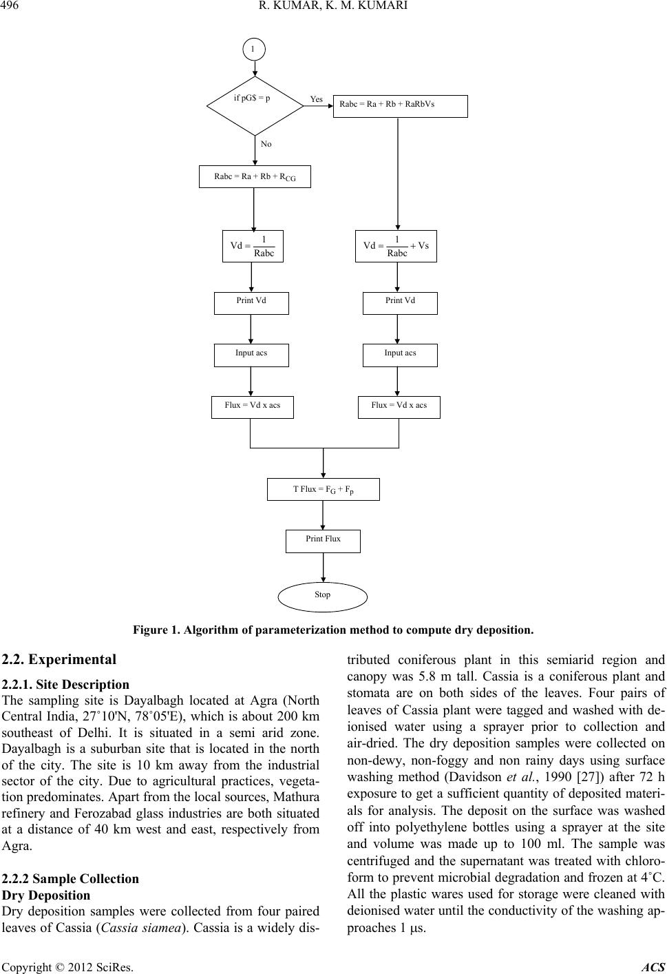


R. KUMAR, K. M. KUMARI
496
Yes Rabc = Ra + Rb + RaRbVs
No
Rabc = Ra + Rb + R
CG
Rabc
1
Vd Vs
Rabc
1Vd 
Print Vd Print Vd
Input acs Input acs
Flux = Vd x acs Flux = Vd x acs
T Flux = F
G
+ F
p
Print Flux
Stop
if pG$ = p
1
Figure 1. Algorithm of parameterization method to compute dry deposition.
2.2. Experimental
2.2.1. Site Description
The sampling site is Dayalbagh located at Agra (North
Central India, 27˚10'N, 78˚05'E), which is about 200 km
southeast of Delhi. It is situated in a semi arid zone.
Dayalbagh is a suburban site that is located in the north
of the city. The site is 10 km away from the industrial
sector of the city. Due to agricultural practices, vegeta-
tion predominates. Apart from the local sources, Mathura
refinery and Ferozabad glass industries are both situated
at a distance of 40 km west and east, respectively from
Agra.
2.2.2 Sample Collection
Dry Deposition
Dry deposition samples were collected from four paired
leaves of Cassia (Cassia siamea). Cassia is a widely dis-
tributed coniferous plant in this semiarid region and
canopy was 5.8 m tall. Cassia is a coniferous plant and
stomata are on both sides of the leaves. Four pairs of
leaves of Cassia plant were tagged and washed with de-
ionised water using a sprayer prior to collection and
air-dried. The dry deposition samples were collected on
non-dewy, non-foggy and non rainy days using surface
washing method (Davidson et al., 1990 [27]) after 72 h
exposure to get a sufficient quantity of deposited materi-
als for analysis. The deposit on the surface was washed
off into polyethylene bottles using a sprayer at the site
and volume was made up to 100 ml. The sample was
centrifuged and the supernatant was treated with chloro-
form to prevent microbial degradation and frozen at 4˚C.
All the plastic wares used for storage were cleaned with
deionised water until the conductivity of the washing ap-
proaches 1 s.

R. KUMAR, K. M. KUMARI 497
Measurements in Air
Particulate
Aerosol samples were collected with KIMOTO (CPS-
105) 4 stage size segregated impactor using high volume
sampler (HVS) equipped with automatic flow rate con-
troller at a flow rate of 1000 L·min–1. The impactor sepa-
rates particles in air according to their aerodynamic di-
ameter. Predesiccated and preweighed Whatman 41 fil-
ters were used as collecting surface. After 24 h collection
period, filters were withdrawn and kept in desiccators.
Each filter was extracted in 100 ml deionized water for
two hours, kept on ultrasonic bath for half an hour and
then filtered through Whatman 41 paper into polyethyl-
ene bottles. Samples were treated in the similar manner
as dry deposition samples and stored under refrigeration
till analysis.
Vapour Phase
Gaseous SO2 was collected by impinger technique us-
ing a low volume sampler comprising a diaphragm re-
ciprocating type of air pump (Model Dymax 2, Charles
Austin Pvt. Ltd., England). SO2 samples were collected
by aspirating air through measured volume (50 ml) of
0.04 M potassium tetrachloromercurate (K2HgCl4) (TCM)
solution at a flow rate of 2 L·min–1 for 24 h. SO2 was
estimated by West and Gaeke method (Harrison and
Perry, 1986 [28]).
2.3. Analysis
2
SO 
2
SO
4 in dry deposition and aerosol samples were mea-
sured by Ion chromatography using a Dionex DX-500
Ion chromatograph system equipped with guard column
(AS 11A), separator column (AS 11ASC), self regener-
ating suppressor (SRS) and conductivity detector (CD-20)
using 5.5 mM NaOH as eluent at flow rate of 1 ml·m–1.
Vapor phase SO2 was analyzed by UV-Visible Spectro-
photometer (Shimadzu Model-1601).
2.4. Meteorological Parameters
The meteorological parameters viz., temperature, relative
humidity, wind speed, wind direction and solar radiation
were monitored at Dayalbagh using a self contained bat-
tery operated WDL 1002 Data logger (Dynalab, Pune)
system. Table 3 presents the sensors used along with
resolution and accuracy of meteorological parameters.
The data was collected for the study period July 1999 to
June 2001. Arithmetic mean, standard deviation, mini-
mum and maximum of meteorological parameters, which
are used for model calculation, are presented in Table 4.
2.5. Uncertainty (Experimental and Analytical)
As a careful analysis of errors is essential in an experi-
ment of present type, numerous calibrations including
collection of field blank, repeatability, instruments ana-
lytical precision, accuracy and detection limits etc. have
been done.
1) The instrument Dionex DX-500 Ion Chromatograph
was calibrated daily with fresh working standard solution
of 2 ppm, prepared daily from 1000 ppm stock standard
solutions of 4

. Although the standard peak heights
never changed by more than a few percent throughout the
day and the variation in peak area was found to be less
than 5%; instrument was recalibrated after every five
samples.
2) Analytical uncertainties arise from the non-ideal
chemical or physical behavior of analytical systems.
The term precision is used to describe the reproduci-
bility of results. In order to calculate the precision a
standard of 1 ppm was run for nine times and the preci-
sion reported as deviation from the mean in terms of
percentage.
The term accuracy denotes the nearness of a meas-
urement to its accepted value and is expressed in terms of
error. The accuracy was calculated by the difference be-
tween observed value Xo and the accepted value Xa.
A = Xo − Xa
In this expression the accepted value may itself be
subjected to considerable uncertainty so the more realis-
tic term is relative error, which is error in terms of per-
centage. The accuracy has been calculated in terms of
relative errors (%). Analytical precision, accuracy and
detection limits of instruments for are 1.1%, 6.3%
and 0.12 µg·l–1, respectively.
2
4
SO 
3) Field blank for dry deposition to leaf surfaces were
collected in the same manner as dry deposition samples
by exposing leaves for one minute to see the ion leakage
during washing (leaching) the leaves. The samples of
field blank were treated and analyzed and were found to
be below detection limit.
4) Field blanks for particulate samples were also col-
lected by mounting the Whatman filter paper in the sam-
pler and putting the system on just for 1 minute. The con-
centration of analytes was found to be close to detection
limits. Field blank for vapor phase SO2 was collected for
one minute following the same procedure as for sample
Table 3. Sensors used, resolution and accuracy of meteoro-
logical parameters.
Measurement
Parameters Sensors Resolution Accuracy Units
Wind speed3 Cup
Anemometer - ±2% m/s
Wind directionWind vane1º ±3º Degree
Relative
humidity
Solid state
capacitive type0.1% 3% of full scale reading % of full scale
Solar radiation72 element
thermopile - - W·m−2
Ambient
temperature
Platinum
resistance 0.1ºC 0.2ºC ºC

R. KUMAR, K. M. KUMARI
Cop2012 SciRes. ACS
498
Table 4. Temperature, relative humidity, solar radiation, wind speed and wind direction of the study period.
Temperature (˚C) Relative humidity (%)Solar Radiation (W·m−2)Wind Speed (m·s−1) Wind Direction
Winter
Arithmetic mean 16.08 70.95 573.13 1.66 W, NW, NE
Standard deviation 3.24 9.88 154.29 0.33 45º
Minimum 11.1 52.3 365.0 1.14
Maximum 23.0 87.8 732.5 2.83
Summer
Arithmetic mean 33.04 51.28 982.08 1.87 W, NW, SW
Standard deviation 3.10 16.31 238.86 0.68 45º
Minimum 25.1 24.1 620.0 0.91
Maximum 39.2 83.0 1330.0 2.56
Monsoon
Arithmetic mean 30.43 71.49 847.94 1.96 W, SW, NW, NE
Standard deviation 1.66 12.20 250.54 0.53 67.5º
Minimum 28.1 45.19 370.0 1.11
Maximum 34.25 86.3 1128.25 2.92
Annual
Arithmetic mean 25.79 63.98 872.73 1.88 NW, W
Standard deviation 8.36 16.09 266.7 0.54 67.5º
Minimum 11.1 24.10 365.0 0.91
Maximum 39.2 87.8 1330.0 2.92
collections. Field blank values for vapor phase were
found to be below detection limit.
Average annual and seasonal atmospheric concentra-
tions of SO2, and 4
2
SO

are presented in Table 6. The
annual mean atmospheric concentration is 3.54 ± 1.41
g·m–3 for SO2 and 2.72 ± 1.15 g m–3 for 4
5) Flow rate in collection of trace gases were corrected
by checking the flow rate by a calibrated rotameter at an
interval of one hour and average values obtained were
considered in the calculation.
2
SO

. The
dry deposition flux of 4 on Cassia leaf is deter-
mined experimentally and annual mean value is 1.07 ±
1.35 mg·m–2·d–1 for SO
2
SO 
2
4

(Table 7). To find out the
deposition of SO2, and 4, the atmospheric concen-
tration of SO2 and 4
3. Results and Discussion 2
SO 
2
SO

were multiplied with their re-
spective deposition velocity to Cassia leaf. The calcu-
lated dry deposition flux of gaseous SO2 is 0.97 ± 0.4
mg· m–2·d–1 and particulate is 1.76 ± 0.74 mg·m–2·
Table 5 presents the values of aerodynamic resistance
(Ra), quassilaminar resistance (Rb), foliar resistance
(Rcf), settling velocity (Vs), and deposition velocity (Vd).
The theoretically calculated dry deposition velocity of
gaseous SO2 ranged between 0.25 to 0.35 and 0.74 to
0.78 cm·s–1 for particulate 4 on Cassia leaf. It has
been seen from the table that dry deposition velocity of
particulate are higher than that of gaseous SO2.
The reported values for dry deposition velocity lie in the
range of 0 to 3.4 cm·s–1 for SO2 (Fowler, 1978 [8]) and
0.01 to 2.9 cm·s–1 for 4
SO
2
SO 
2
SO 
2
SO
4
d–1. In ambient air, rates of oxidation of SO2 up to 30%
h–1 have been observed (Meszaros et al., 1977 [30]; Al-
kenzweeny et al., 1977 [31]). So, 30% of estimated
deposition of SO2, i.e., 0.29 mg·m–2·d–1, would be depos-
ited as sulphate. Depo- sition flux of S as sulphate
(gaseous SO2 + particulate 4) would be 2.05 ± 0.78
mg·m–2·d–1. Experimentally observed dry deposition flux
of 4
2
SO 
2
2
4
SO 

(Nicholson, 1988 [29];
Davidson et al., 1990 [27]). The deposition velocity of
SO2, and fall in the reported range.
2
4

SO

is 1.07 ± 1.35 mg·m–2·d–1, which is compara-
ble to theoretically calculated dry deposition flux of S as
yright ©

R. KUMAR, K. M. KUMARI 499
Table 5. Aerodynamic resistance (Ra), quasilaminar resistance (Rb), stomatal resistance (Rst), mesophyll resistance (Rm), cu-
ticular resistance (Rc), foliar resistance (Rcf), settling velocity (Vs) and deposition velocity (Vd) for gaseous SO2 and particulate
as obtained by parameterization method for Cassia leaf.
2
4
SO 
Species Seasons Aerodynamic
Resistance (Ra)
Quasilaminar
Resistance (Rb)
Combined Stomatal
(Rst) and Mesophyl
Resistance (Rm)
Cuticular
Resistance
(Rcut)*
Coniferous
Resistance (Rcf)
Settling
Velocity (Vs)
Deposition
Velocity (Vd)
SO2 S 0.078 0.96 2.66 100 2.6 NR 0.28
M 0.033 0.96 5.11 100 1.86 NR 0.35
W 0.039 0.96 8.54 100 2.99 NR 0.25
A 0.058 0.96 581 100 2.1 NR 0.32
2
4
SO  S 0.078 1.36 NR NR NR 0.38 1.14
M 0.033 1.36 NR NR NR 0.38 1.18
W 0.039 1.36 NR NR NR 0.38 1.03
A 0.058 1.36 NR NR NR 0.38 1.16
Note: NR = not required. Source: *Seinfeld and Pandis, 1998
2
SO 
2
SO
4 by parameterization method to natural surface
(Table 7).
4. Summary
Dry deposition velocity on natural surface (leaf Cassia
siamea) at Dayalbagh, a suburban site of semiarid region
has been calculated by simulating different processes
governing dry deposition using meteorological data. A
computer program has been developed to make the
method more easy and fast. The calculated dry deposition
velocity by parameterization method for SO2 and 4

are in the reported range. Atmospheric concentration of
Table 6. Atmospheric concentration (g·m−3) of SO2, and
particulate .
2
4
SO 
2
4
SO
SO2

Annual 3.54 ± 1.41 2.72
(1.60 - 6.20) (1.23 - 4.1)
Monsoon 2.72 ± 0.78
(1.60 - 3.50)
3.97 ± 0.71
(2.25 - 4.1)
Winter 4.5 ± 1.45
(2.50 - 6.20)
1.69 ± 0.62
(1.24 - 2.84)
Summer 3.4 ± 1.5
(1.80 - 5.10)
2.51 ± 0.56
(1.23 - 2.96)
Note: The values given in parentheses are range.
Table 7. Experimental and calculated dry deposition flux of
total .
2
4
SO 
2
4
SO 
Species Total
Experimental value 1.07 ± 1.35
(0.06 - 7.86)
Theoretical value 2.05 ± 0.78
(0.92 - 3.17)
gaseous SO2 and particulate 4 were determined and
deposition fluxes were obtained. Dry deposition flux of
4
2
SO 
2
SO

on Cassia leaf has been determined by direct mea-
surement. The dry deposition flux obtained by the current
parameterization method is in the range of dry deposition
flux obtained experimentally on natural surfaces (Cassia
siamea).
5. Acknowledgements
We wish to thank Prof. Satya Prakash, Ex-Head and Prof.
L.D. Khemani, Head, Department of Chemistry and Dr.
K. Hansraj, Department of Mechanical Engineering for
providing help and necessary facilities. The financial
assistance from DST (Project No. SR/FTP/ES-57/2003)
is gratefully acknowledged. Dr. B.B. Rao, Princiapl,
Technical College of the Institute is gratefully acknowl-
edged for kind encouragements.
REFERENCES
[1] P. J. Hanson and S. E. Lindberg, Atmospheric Environ-
ment, Vol. 25A, No. 8, 1991, pp. 1615-1634.
[2] R. Delmas and J. Serrvant, In: H. Rodhe and R. Herrera,
Eds. Acidification in Tropical Countries, 1988, Wiley,
Chichester, pp. 43-72.
[3] J. N. Galloway, G. E. Likens and M. E. Hawley, Science
1984, Vol. 226, pp. 829-831.
[4] B. B. Hicks, D. D. Baldocchi, T. P. Meyers, R. P. Hosker
Jr. and D. R. Matt, “A Preliminary Multiple Resistance
Routine for Deriving Dry Deposition Velocities from
Measured Quantities,” Water, Air and Soil Pollution, Vol.
36, No. 3-4, 1987, pp. 311-330. doi:10.1007/BF00229675
[5] A. S. Thom, In: J. L. Monteith, Ed. Vegetation and At-
mosphere, Academic Press, London, 1975, pp. 58-109.
[6] J. A. Garland, “The Dry Deposition of Sulphur Dioxide to

R. KUMAR, K. M. KUMARI
500
Land and Water Surfaces,” Proceedings of the Royal So-
ciety (A), Vol. 354, No. 1678, 1977, pp. 245-268.
doi:10.1098/rspa.1977.0066
[7] M. L. Wesley and B. B. Hicks, “Some Factors that Affect
the Deposition Rates of Sulfur Dioxide and Similar Gases
on Vegetation,” Journal of Air Pollution Control Asso-
ciation, Vol. 27, No. 11, 1977, pp. 1110-1116.
doi:10.1080/00022470.1977.10470534
[8] D. Fowler, “Dry Deposition of SO2 on Agricultural
Crops,” Atmospheric Environment, Vol. 12, No. 1-3, 1978,
pp. 369-373. doi:10.1016/0004-6981(78)90219-6
[9] J. A. Businger, “Evaluation of the Accuracy with Which
Dry Deposition Can Be Measured with Current Micro-
meteorological Techniques,” Journal of Applied Meteor-
ology, Vol. 25, 1986, pp. 1100-1124.
doi:10.1175/1520-0450(1986)025<1100:EOTAWW>2.0.
CO;2
[10] J. H. Seinfeld and S. N. Pandis, “Atmospheric Chemistry
and Physics: From Air Pollution to Climate Change,”
John Wiley and Sons Inc., Hoboken, 1998.
[11] M. L. Wesley and B. B. Hicks, Atmospheric Environment
2000, Vol. 34, pp. 2261-2282.
[12] J. E. Pleim, A. Venkatram and R. J. Yamartino,
“ADOM/TADAP Model Development Program: The dry
Deposition Module,” Ontario Ministry of Environment,
Rexdale, 1984, p. 4.
[13] J. Padro and G. C. Edwards, Atmospheric-Ocean, Vol. 29,
1991, pp. 667-685.
[14] J. Padro, “Summary of Ozone Dry Deposition Velocity
Measurements and Model Estimates over Vineyard, Cot-
ton, Grass and Deciduous Forest in Summer,” Atmos-
pheric Environment, Vol. 30, No. 13, 1996, pp. 2363-
2369. doi:10.1016/1352-2310(95)00352-5
[15] J. S. Chang, R. A. Brost, S. A. Isaksen, S. Madronich, P.
Middleton, W. R. Stockwell and J. Walcek, Journal of
Geophysical Research, Vol. 92, No. 14, 1987, pp. 681-700.
[16] C. J. Walcek, R. A. Brost, J. S. Chang and M. L. Wesley,
Atmospheric Environment, Vol. 20, 1986, pp. 949-964.
[17] M. L. Wesely, Atmospheric Environment, Vol. 23, No. 6,
1989, pp. 1293-1304.
[18] J. L. Walmsley and M. L. Wesely, Atmospheric Envi-
ronment, Vol. 30, 1996, 1181-1188.
[19] J. W. Erisman and G. P. J. Draaijers, “Atmospheric Depo-
sition in Relation to Acidification and Eutrophication,”
New York, Elsevier, 1995.
[20] E. C. Voldner, L. A. Barrie and A. Sirois, Atmospheric
Environment, Vol. 20, 1986, pp. 2101-2123.
[21] B. B. Hicks, D. D. Baldocchi, R. P. Hosker Jr., B. A.
Hutchison, D. R. Matt, R. T. McMillen, L. C. Satterfield,
“NOAA Technical Memorandum ERL ARL-141,” 1985,
pp. 1-65.
[22] T. P. Meyers and D. D. Baldocchi, Tellus, Vol. 40B, 1988,
pp. 270-284.
[23] D. R. Matt and J. D. Womack, Proceedings of the quad-
rennial Ozone Symposium 1988 and Tropospheric Ozone
Workshop, A. Deepak Publishing, Hampton, 1989, pp.
490-493.
[24] J. Padro, G. den Hartog and H. H. Neumann, Atmospheric
Environment, Vol. 25A, 1991, pp. 1689-1704.
[25] D. W., Stocker, D. H. Stedman, K. F. Zeller, W. J.
Massman and D. G. Fox, “Fluxes of Nitrogen Oxides and
Ozone Measured by Eddy Correlation over a Shortgrass
Prairie,” Journal of Geophysical Research, Vol. 98, No.
D7, 1993, 12619-12630. doi:10.1029/93JD00871
[26] L. W. A. Van Hove, Thesis, University of Wageningen,
Wageningen, 1989.
[27] C. I. Davidson and Y. L. Wu, In: S. E. Lindberg, A. L.
Page and S. A. Norton, Eds., Acidic Precipitation,
Springer Verlag, New York, 1990, pp. 103-216.
[28] R. M. Harrison and R. Perry, “Handbook of Air Pollution
Analysis,” 2nd Edition, Chapman Hall, New York, 1986.
doi:10.1007/978-94-009-4083-3
[29] K. W. Nicholson, Atomspheric Environment, Vol. 22,
1988, pp. 2653-2666.
[30] E. Meszaros, D. J. Moore and J. P. Lodge Jr., “Sulfur
Dioxide-Sulfate Relationships in Budapest,” Atomspheric
Environment, Vol. 11, No. 4, 1977, pp. 345-349.
doi:10.1016/0004-6981(77)90162-7
[31] A. J. Alkenzweeny and D. C. Powell, “Estimation of
Transformation Rate of SO2 to SO4 from Atmospheric
Concentration Data,” Atmospheric Environment, Vol. 11,
No. 2, 1977, pp. 179-182.
doi:10.1016/0004-6981(77)90223-2