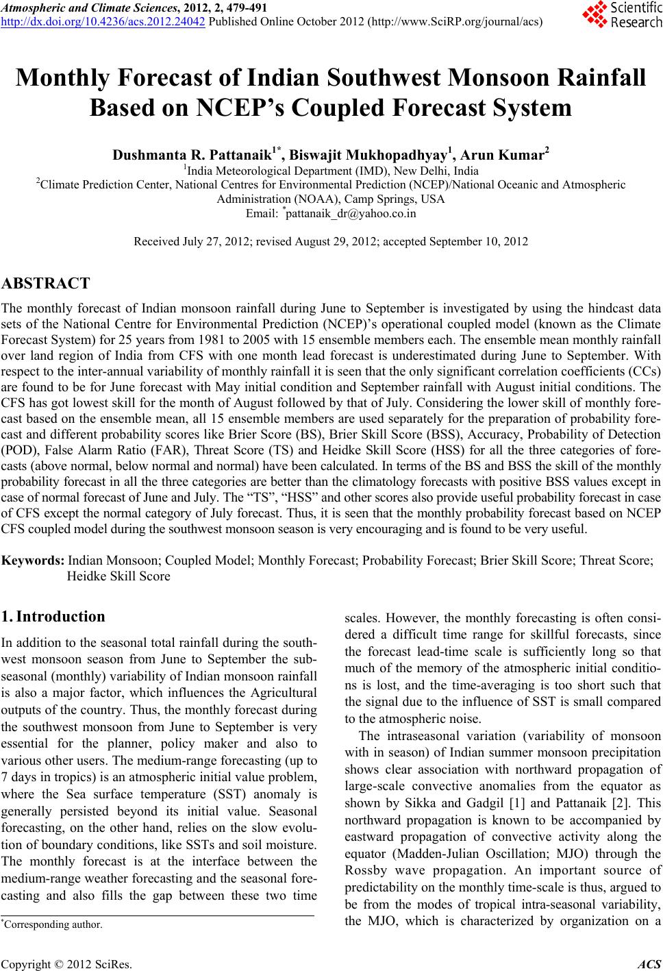
Atmospheric and Climate Sciences, 2012, 2, 479-491
http://dx.doi.org/10.4236/acs.2012.24042 Published Online October 2012 (http://www.SciRP.org/journal/acs)
Monthly Forecast of Indian Southwest Monsoon Rainfall
Based on NCEP’s Coupled Forecast System
Dushmanta R. Pattanaik1*, Biswajit Mukhopadhyay1, Arun Kumar2
1India Meteorological Department (IMD), New Delhi, India
2Climate Prediction Center, National Centres for Environmental Prediction (NCEP)/National Oceanic and Atmospheric
Administration (NOAA), Camp Springs, USA
Received July 27, 2012; revised August 29, 2012; accepted September 10, 2012
ABSTRACT
The monthly forecast of Indian monsoon rainfall during June to September is investigated by using the hindcast data
sets of the National Centre for Environmental Prediction (NCEP)’s operational coupled model (known as the Climate
Forecast System) for 25 years from 1981 to 2005 with 15 ensemble members each. The ensemble mean monthly rainfall
over land region of India from CFS with one month lead forecast is underestimated during June to September. With
respect to the inter-annual variability of monthly rainfall it is seen that the only significant correlation coefficients (CCs)
are found to be for June forecast with May initial condition and September rainfall with August initial conditions. The
CFS has got lowest skill for the month of August followed by that of July. Considering the lower skill of monthly fore-
cast based on the ensemble mean, all 15 ensemble members are used separately for the preparation of probability fore-
cast and different probability scores like Brier Score (BS), Brier Skill Score (BSS), Accuracy, Probability of Detection
(POD), False Alarm Ratio (FAR), Threat Score (TS) and Heidke Skill Score (HSS) for all the three categories of fore-
casts (above normal, below normal and normal) have been calculated. In terms of the BS and BSS the skill of the monthly
probability forecast in all the three categories are better than the climatology forecasts with positive BSS values except in
case of normal forecast of June and July. The “TS”, “HSS” and other scores also provide useful probability forecast in case
of CFS except the normal category of July forecast. Thus, it is seen that the monthly probability forecast based on NCEP
CFS coupled model during the southwest monsoon season is very encouraging and is found to be very useful.
Keywords: Indian Monsoon; Coupled Model; Monthly Forecast; Probability Forecast; Brier Skill Score; Threat Score;
Heidke Skill Score
1. Introduction
In addition to the seasonal total rainfall during the south-
west monsoon season from June to September the sub-
seasonal (monthly) variability of Indian monsoon rainfall
is also a major factor, which influences the Agricultural
outputs of the country. Thus, the monthly forecast during
the southwest monsoon from June to September is very
essential for the planner, policy maker and also to
various other users. The medium-range forecasting (up to
7 days in tropics) is an atmospheric initial value problem,
where the Sea surface temperature (SST) anomaly is
generally persisted beyond its initial value. Seasonal
forecasting, on the other hand, relies on the slow evolu-
tion of boundary conditions, like SSTs and soil moisture.
The monthly forecast is at the interface between the
medium-range weather forecasting and the seasonal fore-
casting and also fills the gap between these two time
scales. However, the monthly forecasting is often consi-
dered a difficult time range for skillful forecasts, since
the forecast lead-time scale is sufficiently long so that
much of the memory of the atmospheric initial conditio-
ns is lost, and the time-averaging is too short such that
the signal due to the influence of SST is small compared
to the atmospheric noise.
The intraseasonal variation (variability of monsoon
with in season) of Indian summer monsoon precipitation
shows clear association with northward propagation of
large-scale convective anomalies from the equator as
shown by Sikka and Gadgil [1] and Pattanaik [2]. This
northward propagation is known to be accompanied by
eastward propagation of convective activity along the
equator (Madden-Julian Oscillation; MJO) through the
Rossby wave propagation. An important source of
predictability on the monthly time-scale is thus, argued to
be from the modes of tropical intra-seasonal variability,
the MJO, which is characterized by organization on a
*Corresponding author.
C
opyright © 2012 SciRes. ACS

D. R. PATTANAIK ET AL.
480
global spatial scale with a period typically ranging from
30 - 60 days [3-6]. Some observational studies of the
northward propagating convective bands associated with
fluctuation of intra-seasonal monsoon activity have been
demonstrated by many studies [1,2,7]. An accurate
coupling of the fast atmosphere to the slow ocean (with
long memory) is essential to simulate the MJO, which in
turn can simulate the intra-seasonal variability of Indian
monsoon.
The monthly forecast using dynamical model was
triggered by the result of the study [8], where they
showed how the pronounced blocking event of 1977 was
successfully reproduced in 1-month forecasts by some
general circulation models. Some of the recent studies
have highlighted that the coupled models with one-tier
approach can enhance the predictability of the summer
monsoon precipitation [9,10]. As shown by Krishnan et
al. [10], a fully coupled model will be able to better
capture the observed monsoon inter-annual variability.
Thus, the future climate prediction system should focus
with coupled atmosphere-ocean models particularly for
the extended range prediction covering the monthly
forecast, which require a better representation of air-sea
interaction and the coupled atmospheric-ocean phenome-
non like MJO in the model.
The leading modeling centres like the European Centre
for Medium range Weather Forecasting (ECMWF) and
the National Centre for Environmental Prediction (NCEP)
have also introduced General Circulation Model and
coupled atmosphere-ocean models operationally for
monthly forecast of atmospheric and oceanic compone-
nts (see Ferranti et al. [11] & Vitart [12] for ECMWF
and Saha et al. [13] for NCEP). As discussed by Vitart
[12] the ECMWF has a dedicated monthly forecasting
system, which was based on 32-day coupled ocean-atm-
osphere integrations run routinely since March 2002.
Though the model is integrated for 32 days the forecast is
prepared on weekly basis valid for days 5 - 11, days 12 -
18, days 19 - 25 and days 26 - 32. As shown by him the
model displays some skill in predicting weekly averaged
2-m temperature, precipitation, and mean sea level
pressure anomalies relative to the climate of the past 12
years. The NCEP coupled modeling system (Known as
the Climate Forecast System (CFS)) on the other hand is
used for both monthly as well as the seasonal forecast.
The skill of the NCEP’s CFS coupled modeling system
for the seasonal rainfall over India during June to
September as shown by Pattanaik and Kumar [14] and
Pattanaik et al. [15] show some useful skill. With the
availability of long hindcast data from various centres
using GCMs and coupled GCMs, a number of studies
[16-23] have been carried out to see the performance of
different models for the monsoon prediction over India in
the extended range time scale. Most of these studies have
focused on the simulation of seasonal monsoon rainfall
over India. In the present study the skill of the NCEP
CFS forecast system is assessed with respect to the
monthly forecast solely by the use of a tier-1 retrospec-
tive set of forecasts for 25 years from 1981 to 2005 for
the Indian monsoon rainfall from June to September. The
ensemble members are also considered separately to
prepare the monthly probability forecast during the
period from 1981 to 2005 and the skill of the probability
forecast is also investigated.
2. Details of the Model Hindcast and the
Methodology
The atmospheric component of the CFS is the NCEP
atmospheric GFS model, as of February 2003 [24]. The
atmospheric component is having a spectral triangular
truncation of 62 waves (T62) in the horizontal and a
finite differencing in the vertical with 64 sigma layers.
This version of the GFS has been modified from the
version of the NCEP model used for the NCEP/NCAR
Reanalysis by Kalnay et al. [25] and Kistler et al. [26],
with upgrades in the parameterization of solar radiation
transfer [27,28], boundary layer vertical diffusion [29],
cumulus convection [30], gravity wave drag [31]. The
oceanic component is the GFDL Modular Ocean Model
V.3 (MOM3), which is a finite difference version of the
ocean primitive equations under the assumptions of Bou-
ssinesq and hydrostatic approximations [32]. It uses
spherical coordinates in the horizontal with a staggered
Arakawa B grid and the z-coordinate in the vertical. The
ocean surface boundary is computed as an explicit free
surface. The domain is quasi-global extending from 74˚S
to 64˚N. The zonal resolution is 1˚. The meridional reso-
lution is 1/3˚ between 10˚S and 10˚N, gradually incre-
asing through the tropics until becoming fixed at 1˚
poleward of 30˚S and 30˚N. There are 40 layers in the
vertical with 27 layers in the upper 400 m, and the
bottom depth is around 4.5 Km. Vertical mixing follows
the non-local K-profile parameterization of Large et al.
[33]. The horizontal mixing of momentum uses the
nonlinear scheme of Smagorinsky [34]. The ocean-
atmosphere coupling is nearly global (64˚N - 74˚S),
instead of only in the tropical Pacific Ocean, and flux
correction is no longer applied. Thus, the CFS is a fully
“tier-1” forecast system. The coupling over the global
ocean required an important upgrade in the ocean data
assimilation as well. An extensive set of retrospective
forecasts (“hindcasts”) was generated to cover a 25 years
period (1981-2005), in order to obtain a history of the
model. This history can be used operationally to calibrate
and assess the skill of the real-time forecasts.
The CFS includes a comprehensive set of retrospective
runs that are used to calibrate and evaluate the skill of its
forecasts. Each run is a full nine month integration with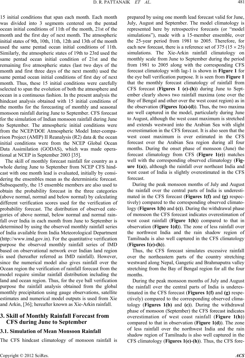

D. R. PATTANAIK ET AL. 481
15 initial conditions that span each month. Each month
was divided into 3 segments centered on the pentad
ocean initial conditions of 11th of the month, 21st of the
month and the first day of next month. The atmospheric
initial states of 9th, 10th, 11th, 12th and 13th of the month
used the same pentad ocean initial conditions of 11th.
Similarly, the atmospheric states of 19th to 23rd used the
same pentad ocean initial condition of 21st and the
remaining five atmospheric states (last two days of the
month and first three days of the next month) used the
same pentad ocean initial conditions of first day of next
month. Thus, these 15 initial conditions were carefully
selected to span the evolution of both the atmosphere and
ocean in a continuous fashion. In the present analysis the
hindcast analysis obtained with 15 initial conditions of
the months for the forecasting of monthly and seasonal
monsoon rainfall during June to September. CFS forecast
for the simulation of Indian monsoon rainfall during June
to September. The atmospheric initial conditions were
from the NCEP/DOE Atmospheric Model Inter-compa-
rison Project (AMIP) II Reanalysis (R2) data & the ocean
initial conditions were from the NCEP Global Ocean
Data Assimilation (GODAS), which was made opera-
tional at NCEP in September 2003 [35].
The skill of monthly forecast rainfall for country as a
whole during June to September from NCEP CFS hind-
cast with one month lead is evaluated, initially by consi-
dering the ensembles mean as the deterministic forecast.
Subsequently, the 15 ensemble members are also used to
obtain the probability forecast in the three categories
(above normal, normal and below normal) by calculating
different verification scores used for the verification of
probability forecast. The distribution of observed cate-
gories of above normal, below normal and normal rain-
fall over India in each month from June to September is
determined by using the observed monthly rainfall series
of India available from India Meteorological Department
(http://www.imd.gov.in). For the quantitative verification
purpose the observed monthly rainfall series of IMD
based on observational network over Indian land region
is used (hereafter referred as IMD rainfall). However,
since the numerical model also gives rainfall over the
Ocean region the verification of rainfall forecast from the
model require similar rainfall distribution including the
land and ocean region. Thus, for the eye ball verification
purpose the rainfall analysis obtained from the global
monthly precipitation using gauge observations, satellite
estimates and numerical model outputs is used from Xie
and Arkin, [36]; hereafter known as Xie-Arkin rainfall.
3. Skill of Monthly Rainfall Forecast from
CFS during June to September
3.1. Simulation of Mean Monsoon Rainfall
The CFS hindcast climatology of monsoon rainfall is
prepared by using one month lead forecast valid for June,
July, August and September. The model climatology is
represented here by retrospective forecasts (or “model
simulations”), made with a 15-member ensemble, over
the 25-year period from 1981 to 2005. Therefore, for
each new forecast, there is a reference set of 375 (15  25)
simulations. The Xie-Arkin rainfall climatology on
monthly scale from June to September during the period
from 1981 to 2005 along with the corresponding CFS
forecast climatology with lag-1 is shown in Figure 1 for
the eye ball verification purpose. It is seen from Figure 1
that the monthly forecast climatology of rainfall from
CFS forecast (Figures 1 (e)-(h)) during June to Sept-
ember clearly shows two rainfall maxima (one over the
Bay of Bengal and other over the west coast region) as in
the observation (Figures 1(a)-(d)). Thus, the two maxima
are well captured in the model, particularly during June
to August, although the west coast maximum is stretched
and extends westward into the Arabian Sea with slight
overestimation in the CFS forecast. It is also seen that the
west coast maximum is over estimated in the CFS
forecast over the Arabian Sea region during all four
months. During the onset phase of monsoon (June) the
forecast climatology from CFS (Figure 1(e)) matches
well with the corresponding observed climatology (Fig-
ure 1(a)), although the rainfall over northeast India and
west coast of India is slightly overestimated in the CFS
forecast.
During the peak monsoon months of July and August
the rainfall over the central parts of India is underesti-
mated in the CFS forecast (Figures 1(f) and (g) respec-
tively) compared to the corresponding observed climato-
logy (Figures 1(b) and (c)). During the withdrawal phase
of monsoon the CFS forecast indicates overestimation of
west coast rainfall (Figure 1(h)) compared to that in
observation (Figure 1(d)). The zone of less rainfall over
the northwest India and the rain shadow region of
Tamilnadu is also well captured in the CFS climatology
(Figures 1(e)-(h)).
Thus, the CFS forecast simulates excessive rainfall
over the northeastern parts of the country stretching
westward along Nepal, Gangetic and Brahmaputra valley
stretching from the Bay of Bengal region for all the four
months.
During the peak monsoon months of July and August
the rainfall over the central parts of India is underes-
timated in the CFS forecast (Figures 1(f) and (g) respe-
ctively) compared to the corresponding observed clima-
tology (Figures 1(b) and (c)). During the withdrawal
phase of monsoon (September) the CFS forecast indicates
overestimation of west coast rainfall (Figure 1(h))
compared to that in observation (Figure 1(d)). The zone
of less rainfall over the northwest India and the rain
shadow region of Tamilnadu is also well captured in the
CFS climatology (Figures 1(e)-(h)). Thus, the CFS fore-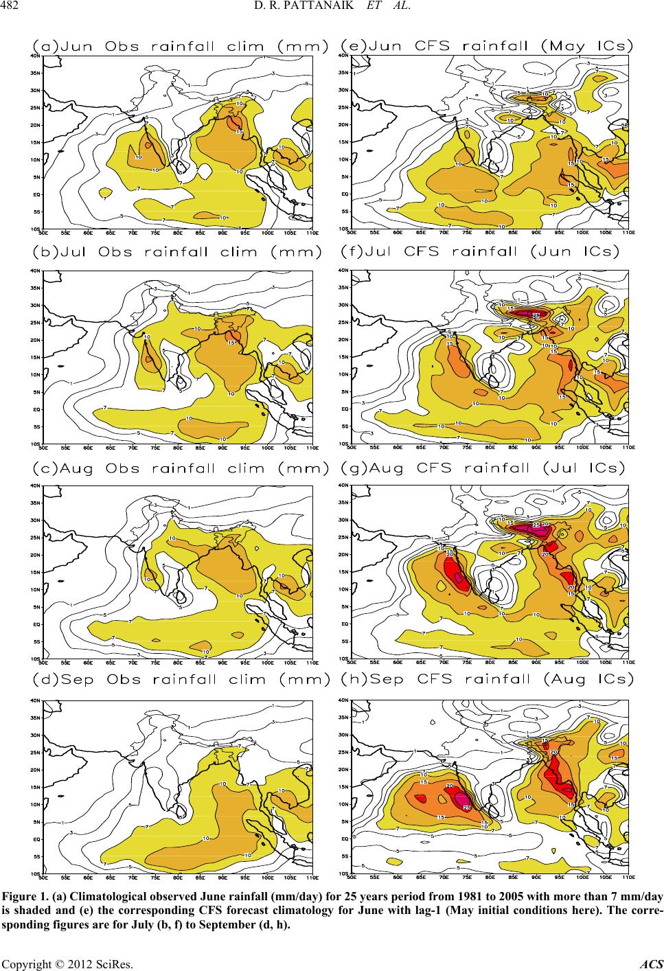

D. R. PATTANAIK ET AL.
482
Figure 1. (a) Climatological observed June rainfall (mm/day) for 25 years period from 1981 to 2005 with more than 7 mm/day
is shaded and (e) the corresponding CFS forecast climatology for June with lag-1 (May initial conditions here). The corre-
sponding figures are for July (b, f) to September (d, h).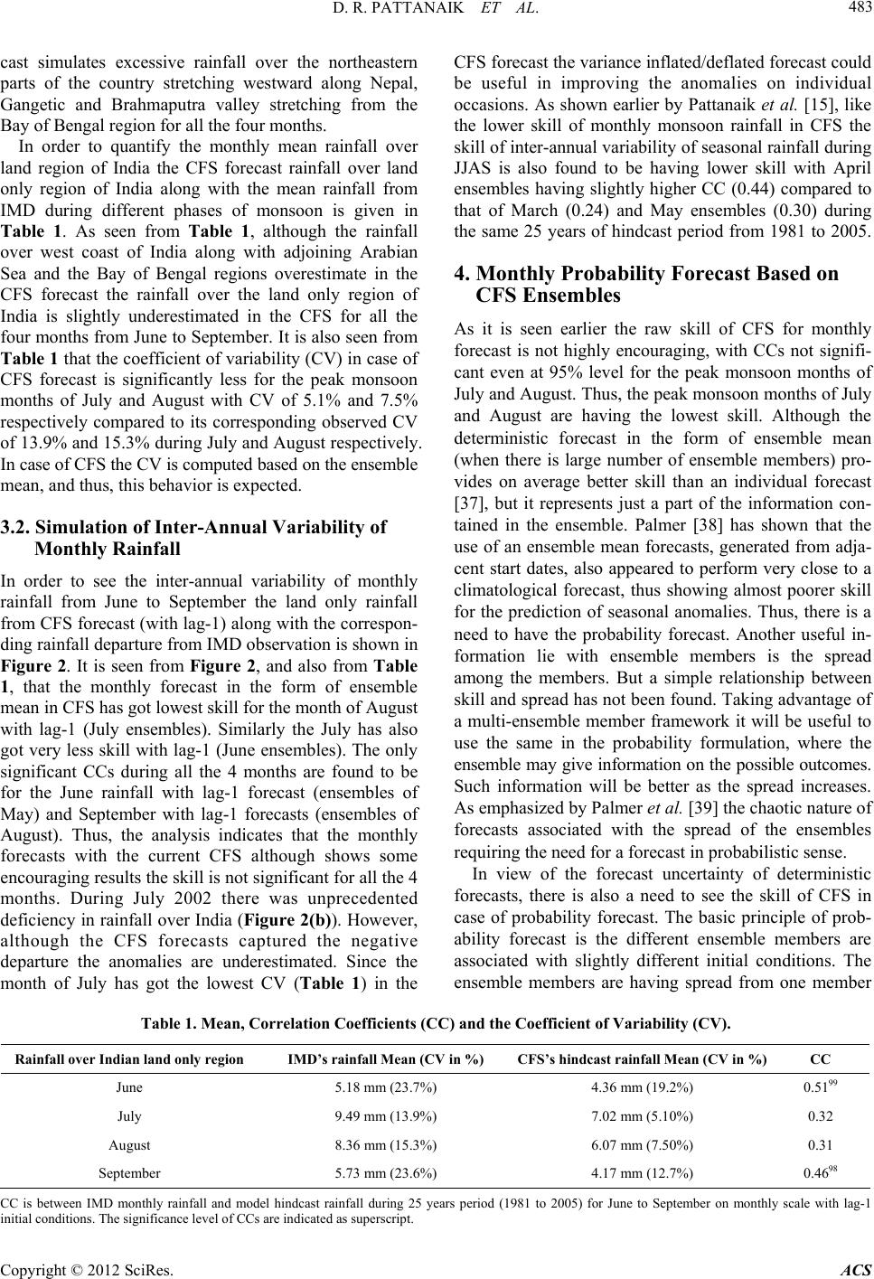

D. R. PATTANAIK ET AL. 483
cast simulates excessive rainfall over the northeastern
parts of the country stretching westward along Nepal,
Gangetic and Brahmaputra valley stretching from the
Bay of Bengal region for all the four months.
In order to quantify the monthly mean rainfall over
land region of India the CFS forecast rainfall over land
only region of India along with the mean rainfall from
IMD during different phases of monsoon is given in
Table 1. As seen from Table 1, although the rainfall
over west coast of India along with adjoining Arabian
Sea and the Bay of Bengal regions overestimate in the
CFS forecast the rainfall over the land only region of
India is slightly underestimated in the CFS for all the
four months from June to September. It is also seen from
Table 1 that the coefficient of variability (CV) in case of
CFS forecast is significantly less for the peak monsoon
months of July and August with CV of 5.1% and 7.5%
respectively compared to its corresponding observed CV
of 13.9% and 15.3% during July and August respectively.
In case of CFS the CV is computed based on the ensemble
mean, and thus, this behavior is expected.
3.2. Simulation of Inter-Annual Variability of
Monthly Rainfall
In order to see the inter-annual variability of monthly
rainfall from June to September the land only rainfall
from CFS forecast (with lag-1) along with the correspon-
ding rainfall departure from IMD observation is shown in
Figure 2. It is seen from Figure 2, and also from Table
1, that the monthly forecast in the form of ensemble
mean in CFS has got lowest skill for the month of August
with lag-1 (July ensembles). Similarly the July has also
got very less skill with lag-1 (June ensembles). The only
significant CCs during all the 4 months are found to be
for the June rainfall with lag-1 forecast (ensembles of
May) and September with lag-1 forecasts (ensembles of
August). Thus, the analysis indicates that the monthly
forecasts with the current CFS although shows some
encouraging results the skill is not significant for all the 4
months. During July 2002 there was unprecedented
deficiency in rainfall over India (Figure 2(b)). However,
although the CFS forecasts captured the negative
departure the anomalies are underestimated. Since the
month of July has got the lowest CV (Table 1) in the
CFS forecast the variance inflated/deflated forecast could
be useful in improving the anomalies on individual
occasions. As shown earlier by Pattanaik et al. [15], like
the lower skill of monthly monsoon rainfall in CFS the
skill of inter-annual variability of seasonal rainfall during
JJAS is also found to be having lower skill with April
ensembles having slightly higher CC (0.44) compared to
that of March (0.24) and May ensembles (0.30) during
the same 25 years of hindcast period from 1981 to 2005.
4. Monthly Probability Forecas t Based on
CFS Ensembles
As it is seen earlier the raw skill of CFS for monthly
forecast is not highly encouraging, with CCs not signifi-
cant even at 95% level for the peak monsoon months of
July and August. Thus, the peak monsoon months of July
and August are having the lowest skill. Although the
deterministic forecast in the form of ensemble mean
(when there is large number of ensemble members) pro-
vides on average better skill than an individual forecast
[37], but it represents just a part of the information con-
tained in the ensemble. Palmer [38] has shown that the
use of an ensemble mean forecasts, generated from adja-
cent start dates, also appeared to perform very close to a
climatological forecast, thus showing almost poorer skill
for the prediction of seasonal anomalies. Thus, there is a
need to have the probability forecast. Another useful in-
formation lie with ensemble members is the spread
among the members. But a simple relationship between
skill and spread has not been found. Taking advantage of
a multi-ensemble member framework it will be useful to
use the same in the probability formulation, where the
ensemble may give information on the possible outcomes.
Such information will be better as the spread increases.
As emphasized by Palmer et al. [39] the chaotic nature of
forecasts associated with the spread of the ensembles
requiring the need for a forecast in probabilistic sense.
In view of the forecast uncertainty of deterministic
forecasts, there is also a need to see the skill of CFS in
case of probability forecast. The basic principle of prob-
ability forecast is the different ensemble members are
associated with slightly different initial conditions. The
ensemble members are having spread from one member
Table 1. Mean, Correlation Coefficients (CC) and the Coefficient of Variability (CV).
Rainfall over Indian land only region IMD’s rainfall Mean (CV in %) CFS’s hindcast rainfall Mean (CV in %) CC
June 5.18 mm (23.7%) 4.36 mm (19.2%) 0.5199
July 9.49 mm (13.9%) 7.02 mm (5.10%) 0.32
August 8.36 mm (15.3%) 6.07 mm (7.50%) 0.31
September 5.73 mm (23.6%) 4.17 mm (12.7%) 0.4698
CC is between IMD monthly rainfall and model hindcast rainfall during 25 years period (1981 to 2005) for June to September on monthly scale with lag-1
initial conditions. The significance level of CCs are indicated as superscript.

D. R. PATTANAIK ET AL.
484
-40
-30
-20
-10
0
10
20
30
40
1981 1982 1983 1984 1985 1986 1987 1988 1989 1990 1991 1992 1993 1994 1995 1996 1997 1998 1999 2000 2001 2002
year
% De p of m onthly rainfall
2003 2004 2005
CFS Jun RF (May, CC=0.51)
IMD Jun RF
(a)
(a)
-60
-50
-40
-30
-20
-10
0
10
20
30
40
1981 1982 1983 1984 1985 1986 1987 1988 1989 1990 1991 1992 1993 1994 1995 1996 1997 1998 1999 2000 2001 2002 2003 2004 2005
y
ear
% D ep of monthly rainfall
CFS Jul RF (Jun, CC=0.32)
IMD Jul RF
(b)
(b)
-30
-20
-10
0
10
20
30
1981 1982 1983 1984 1985 1986 1987 1988 1989 1990 1991 1992 1993 1994 1995 1996 1997 1998 1999 2000 2001 2002
year
% De p of monthly rainfall
2003 2004 2005
CFS Aug RF (Jul, CC=0.31)
IMD Aug RF
(c)
(c)
-50
-40
-30
-20
-10
0
10
20
30
40
50
1981 1982 1983 1984 1985 1986 1987 1988 1989 1990 1991 1992 1993 1994 1995 1996 1997 1998 1999 2000 2001 2002
year
% De p of monthly ra infall
2003 2004 2005
CFS Sep RF (Aug,CC=0.46)
IMD Sep RF
(d)
(d)
Figure 2. (a)Year-to-year variation of % departure of observed June rainfall over India along with that of rainfall from CFS
forecast with one month lead for the month of June over Indian land mass (May ICs); (b), (c) and (d) for observed and CFS
rainfall from July to September respectively.

D. R. PATTANAIK ET AL.
ACS
485
to other. Thus, if the ensemble members have large stan-
dard deviation, which indicates it has large spread or the
ensemble members deviates from one another (good for
the probability forecast). The spread of a variable indi-
cates the forecast diversity of the ensemble mean among
all the members. Small spread indicates low forecast un-
certainty, large spread high forecast uncerta- inty. Large
spread should not be taken as a reason not to issue a
forecast. In that case the best strategy will be to issue a
forecast based on the ensemble mean but to be careful in
the formulations and try to indicate possible alternatives.
The spread will also indicate what is not likely to happen,
which at times might be as important as knowing what is
likely to happen. In order to see the spread of ensemble
members, the 15 individual member monthly forecasts
rainfall averaged over land only region of India with
lag-1 ensemble valid for June to September is shown in
Figure 3. Along with the ensemble members the ensem-
ble spread in the form of Standard Deviation (SD) during
each monthly forecast is also plotted in Figure 3 (in
secondary Y-axis). Thus, the spread is calculated as SD
with respect to ensemble mean for each monthly forecast
separately. As it is seen from Figure 3(a) the forecast for
June rainfall during the period from 1981 to 2005 shows
large spread of ensemble members in most of the years
with mean SD is found to be 1.15 mm/day (Figure 3(a)).
However, the month of July and August have got the
lower spread among the members, which indicates the
members are closer to the ensemble mean. The mean SD
for July and August during the 25 years period as seen
from Figures 3(b) and (c) is found to be 0.86 mm/day
and 0.90 mm/day respectively. For the month of Sep-
tember as seen from Figure 3(d) it is seen that the en-
semble spread is slightly higher than that during July and
August with mean SD during the 25 years period
(1981-2005) is found to be 0.98 mm/day. The spread of
the ensemble members in case of monthly forecast for all
4 months are the basis of preparing monthly probability
forecast.
There are different methods of generating probability
forecasts. Based on the ensemble members the probabil-
ity of above normal, below normal or normal may be
calculated at each grid point by using the climatological
information of CFS hindcast over the region for 25 years
(a) June (May IC) (b) July (Jun IC)
(c) August (Jul IC) (d) September (August IC)
Figure 3. (a) Maximum, minimum and mean values of the 15 ensemble members of the forecast for June along with the en-
semble spread (in terms of standard deviation) during the period from 1981 to 2005; (b) Same as “a” but for July; (c) Same
as “a” but for August; (d) Same as “a” but for September.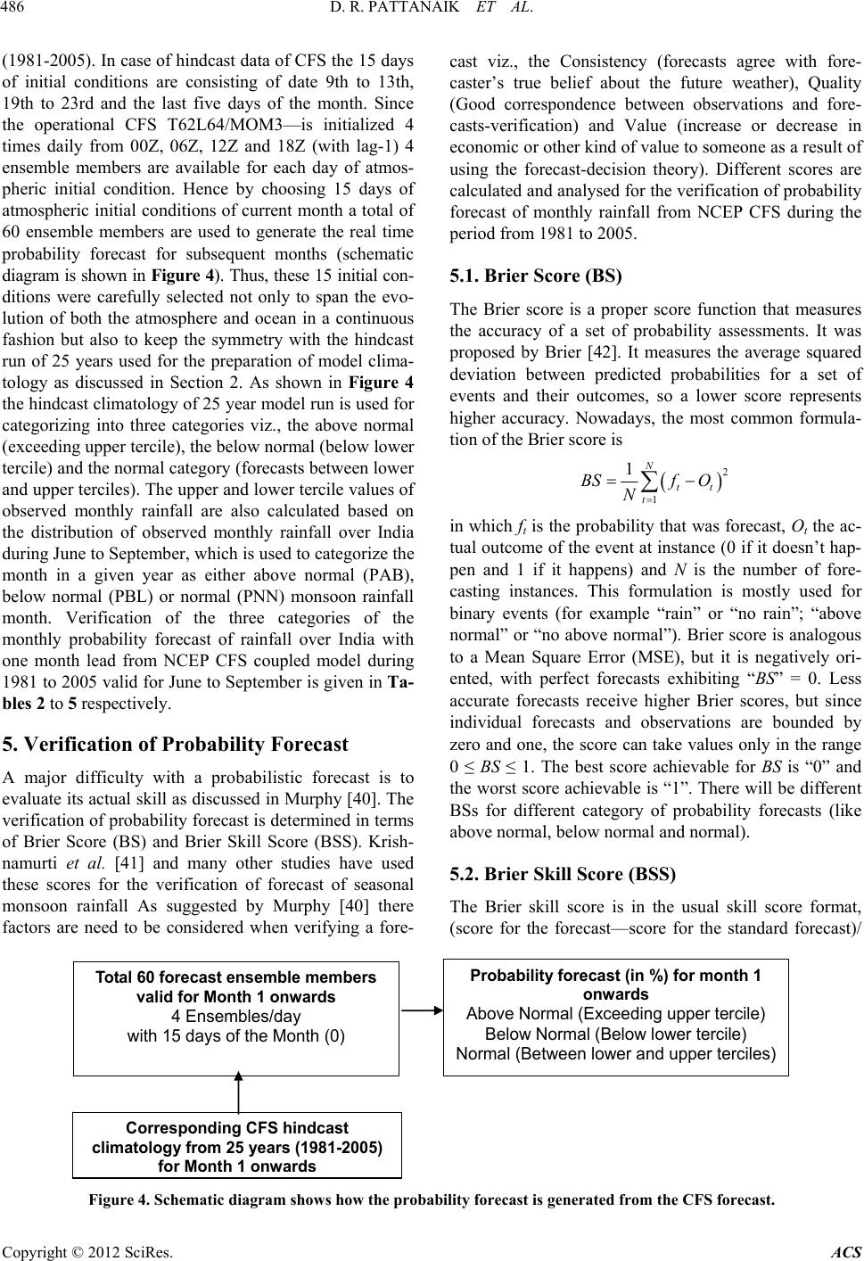

D. R. PATTANAIK ET AL.
486
(1981-2005). In case of hindcast data of CFS the 15 days
of initial conditions are consisting of date 9th to 13th,
19th to 23rd and the last five days of the month. Since
the operational CFS T62L64/MOM3—is initialized 4
times daily from 00Z, 06Z, 12Z and 18Z (with lag-1) 4
ensemble members are available for each day of atmos-
pheric initial condition. Hence by choosing 15 days of
atmospheric initial conditions of current month a total of
60 ensemble members are used to generate the real time
probability forecast for subsequent months (schematic
diagram is shown in Figure 4). Thus, these 15 initial con-
ditions were carefully selected not only to span the evo-
lution of both the atmosphere and ocean in a continuous
fashion but also to keep the symmetry with the hindcast
run of 25 years used for the preparation of model clima-
tology as discussed in Section 2. As shown in Figure 4
the hindcast climatology of 25 year model run is used for
categorizing into three categories viz., the above normal
(exceeding upper tercile), the below normal (below lower
tercile) and the normal category (forecasts between lower
and upper terciles). The upper and lower tercile values of
observed monthly rainfall are also calculated based on
the distribution of observed monthly rainfall over India
during June to September, which is used to categorize the
month in a given year as either above normal (PAB),
below normal (PBL) or normal (PNN) monsoon rainfall
month. Verification of the three categories of the
monthly probability forecast of rainfall over India with
one month lead from NCEP CFS coupled model during
1981 to 2005 valid for June to September is given in Ta-
bles 2 to 5 respectively.
5. Verification of Probability Forecast
A major difficulty with a probabilistic forecast is to
evaluate its actual skill as discussed in Murphy [40]. The
verification of probability forecast is determined in terms
of Brier Score (BS) and Brier Skill Score (BSS). Krish-
namurti et al. [41] and many other studies have used
these scores for the verification of forecast of seasonal
monsoon rainfall As suggested by Murphy [40] there
factors are need to be considered when verifying a fore-
cast viz., the Consistency (forecasts agree with fore-
caster’s true belief about the future weather), Quality
(Good correspondence between observations and fore-
casts-verification) and Value (increase or decrease in
economic or other kind of value to someone as a result of
using the forecast-decision theory). Different scores are
calculated and analysed for the verification of probability
forecast of monthly rainfall from NCEP CFS during the
period from 1981 to 2005.
5.1. Brier Score (BS)
The Brier score is a proper score function that measures
the accuracy of a set of probability assessments. It was
proposed by Brier [42]. It measures the average squared
deviation between predicted probabilities for a set of
events and their outcomes, so a lower score represents
higher accuracy. Nowadays, the most common formula-
tion of the Brier score is

2
1
1N
tt
t
BSf O
N


in which ft is the probability that was forecast, Ot the ac-
tual outcome of the event at instance (0 if it doesn’t hap-
pen and 1 if it happens) and N is the number of fore-
casting instances. This formulation is mostly used for
binary events (for example “rain” or “no rain”; “above
normal” or “no above normal”). Brier score is analogous
to a Mean Square Error (MSE), but it is negatively ori-
ented, with perfect forecasts exhibiting “BS” = 0. Less
accurate forecasts receive higher Brier scores, but since
individual forecasts and observations are bounded by
zero and one, the score can take values only in the range
0 ≤ BS ≤ 1. The best score achievable for BS is “0” and
the worst score achievable is “1”. There will be different
BSs for different category of probability forecasts (like
above normal, below normal and normal).
5.2. Brier Skill Score (BSS)
The Brier skill score is in the usual skill score format,
(score for the forecast—score for the standard forecast)/
Probability forecast (in %) for month 1
onwards
Above Normal (Exceeding upper tercile)
Below Normal (Below lower tercile)
Normal (Between lower and upper terciles)
Total 60 forecast ensemble members
valid for Month 1 onwards
4 Ensembles/day
with 15 days of the Month (0)
Corresponding CFS hindcast
climatology from 25 years (1981-2005)
for Month 1 onwards
Figure 4. Schematic diagram shows how the probability forecast is generated from the CFS forecast.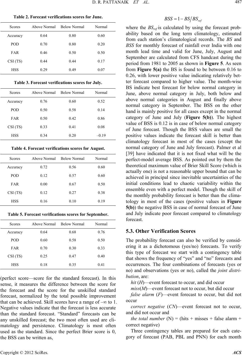

D. R. PATTANAIK ET AL. 487
Table 2. Forecast verifications scores for June.
Scores Above Normal Below Normal Normal
Accuracy 0.64 0.80 0.60
POD 0.70 0.80 0.20
FAR 0.46 0.50 0.50
CSI (TS) 0.44 0.44 0.17
HSS 0.29 0.49 0.07
Table 3. Forecast verifications scores for July.
Scores Above Normal Below Normal Normal
Accuracy 0.76 0.60 0.52
POD 0.50 0.58 0.14
FAR 0.50 0.42 0.86
CSI (TS) 0.33 0.41 0.08
HSS 0.34 0.20 –0.19
Table 4. Forecast verifications scores for August.
Scores Above Normal Below Normal Normal
Accuracy 0.72 0.56 0.60
POD 0.12 0.57 0.60
FAR 0.00 0.67 0.50
CSI (TS) 0.12 0.27 0.38
HSS 0.16 0.10 0.19
Table 5. Forecast verifications scores for September.
Scores Above Normal Below Normal Normal
Accuracy 0.64 0.68 0.76
POD 0.60 0.58 0.50
FAR 0.70 0.30 0.33
CSI (TS) 0.25 0.47 0.40
HSS 0.18 0.35 0.41
(perfect score—score for the standard forecast). In this
sense, it measures the difference between the score for
the forecast and the score for the unskilled standard
forecast, normalized by the total possible improvement
that can be achieved. Skill scores have a range of – to 1.
Negative values indicate that the forecast is less accurate
than the standard forecast. “Standard” forecasts can be
any unskilled forecast; the two most often used are cli-
matology and persistence. Climatology is most often
used as the standard. Since the perfect Brier score is 0,
the BSS can be written as,
1ref BSSBS BS


where the BSref is calculated by using the forecast prob-
ability based on the long term climatology, estimated
from each station’s climatological records. The BS and
BSS for monthly forecast of rainfall over India with one
month lead time and valid for June, July, August and
September are calculated from CFS handcast during the
period from 1981 to 2005 as shown in Figure 5. As seen
from Figure 5(a) the BS is found to be between 0.16 to
0.26, with lower positive value indicating relatively bet-
ter forecast compared to higher value. The month-wise
BS indicate best forecast for below normal category in
June, above normal category in July, both below and
above normal categories in August and finally above
normal category in September. The BSS on the other
hand is mainly positive for all cases except in the normal
category of June and July (Figure 5(b)). The highest
value of BSS is 0.12 is in case of below normal category
of June forecast. Though the BSS values are small the
positive values indicate the forecast skill is better than
climatology forecast in most of the cases (except the
normal category of June and July forecast). Palmer et al
[39] have indicated that it is not fixed what will be the
perfect-model average BSS. As pointed out by them the
theoretical maximum value of Brier Skill Score (which is
actually one) is not a reasonable upper bound that can be
achieved in principal since inevitable uncertainties of the
initial conditions lead to chaotic variability within the
ensemble even with a perfect model. Though the skill of
the monthly probability forecast is better than the clima-
tology in most of the cases (positive values in Figure
5(b)) the negative BSS in case of normal forecast of June
and July indicate poor forecast compared to climatology
forecast.
5.3. Other Verification Scores
The probability forecast can also be verified by consid-
ering it as a dichotomous (yes/no) forecasts. To verify
this type of forecast we start with a contingency table
that shows the frequency of “yes” and “no” forecasts and
occurrences. The four combinations of forecasts (yes or
no) and observations (yes or no), called the joint distri-
bution, are:
hit (H)—event forecast to occur, and did occur
miss(M)—event forecast not to occur, but did occur
false alarm (F)—event forecast to occur, but did not
occur
correct negative (CN)—event forecast not to occur,
and did not occur and
the total number (N) = (hits + misses + false alarm +
correct negative)
Three contingency tables are prepared for each cate-
gory of forecast (PAB, PBL and PNN) for each month

D. R. PATTANAIK ET AL.
488
0.23
0.16
0.26
0.18
0.21
0.26
0.21
0.24
0.21
0.10
0.12
0.14
0.16
0.18
0.20
0.22
0.24
0.26
0.28
JuneJuly August
Monthly Forecast ( Lag - 1 fo recast )
Monthly Forecast Brier Score (BS
0.16
0.26
0.21
Se ptempe r
)
BS (PAB)
BS (PBL)
BS( PNN)
(a)
0.12
0.07
0.04
0.06
0.04
0.00
0.03
-0.04
-0.06
-0.10
-0.05
0.00
0.05
0.10
0.15
JuneJuly August
Mont hl y Forecast ( Lag - 1 f orecast )
Monthly Forecast Brier Skill Score (BSS
)
0.08
0.06
0.04
Se pte mpe r
BSS (P AB)
BSS (P BL)
BSS (P NN)
(b)
Figure 5. (a) Brier Score and (b) Brier Skill Score of the
monthly rainfall forecast over the land region of India with
one month lag based on CFS hindcast during the period
from 1981-2005. The scores are computed for all the three
categories of above normal, below normal and normal.
from June to September by comparing the forecast of
monthly rainfall averaged for the country as a whole
from NCEP CFS with corresponding observed monthly
rainfall over India as a whole. For the quantitative veri-
fication many verification scores can be calculated using
the contingency table such as Accuracy, Probability of
Detection (POD), False Alarm Ration (FAR), Critical
Success Index (CSI) or commonly known as Threat
Score (TS), Heidke Skill Score (HSS) etc. The Relative
Operating Characteristics (ROC) also used for the verifi-
cation of probability forecast by Kharin and Zwiers [43].
The ROC is a representation of the skill of a forecasting
system in which the hit rate and the false-alarm rate are
compared [44,45]. The different verification scores used
in the present study are discussed below:
1) Accuracy (fraction correct) = (H + CN)/N
This gives overall, what fraction of the forecasts were
correct. It is very simple but it is heavily influenced by
most common category, usually “no event” in the case of
rare weather. The range is between “0” to “1” with per-
fect score indicating “1”.
2) Probability of Detection (POD) = H/(H + M)
The range is 0 to 1 with latter for perfect score. The
POD gives, what fraction of the observed “yes” were
correctly forecasts? It is sensitive to hits, but ignores
false alarm.
POD is also very sensitive to the climatological fre-
quency of the event. POD is also an important compo-
nent of the ROC used for probability forecasts.
3) False Alarm Ratio (FAR) = F/(H + F)
This gives what fraction of the predicted “yes” events
actually did not occur and the range is between 0 and 1
with perfect score is “0”. The FAR is sensitive to false
alarms, but ignores misses and is very sensitive to the
climatological frequency of the event. It is always advis-
able to use “POD” and “FAR” in conjunction to one an-
other.
4) Threat score (TS) or also known as Critical Success
Index (CSI) = H/(H + M + F)
This gives how well did the forecast “yes” events cor-
respond to the observed “yes” events? The range is be-
tween “0” and “1” with “0” indicates no skill and “1”
indicates perfect score. CIS measures the fraction of ob-
served and/or forecast events that were correctly pre-
dicted. It can be thought of as the accuracy when correct
negatives have been removed from consideration, that is,
TS is only concerned with forecasts that count. Sensitive
to hits, penalizes both misses and false alarms. Depends
on climatological frequency of events (poorer scores for
rarer events) since some hits can occur purely due to
random chance.
5) Heidke Skill Score (HSS)
The Heidke Skill score is in the usual skill score for-
mat and is defined as = (score value – score for the
standard forecast)/(perfect score – score for the standard
forecast). Or using the contingency Table “HSS” can be
written as






random
random
–expected correct
HSS
–expected correct
HCN
N

 







where (expected correct)random = [(H + M)(H + F) + (CN
+ M)(CN + F)]/N
For the HSS, the “score” is the number correct or the
proportion correct. The “standard forecast” is usually the
number correct by chance or the proportion correct by
chance. The HSS measures the fractional improvement
of the forecast over the standard forecast. Like most skill
scores, it is normalized by the total range of possible im-
provement over the standard, which means HSS can
safely be compared on different datasets. The range of
the HSS is −∞ to 1. Negative values indicate that the
chance forecast is better, “0” means no skill, and a per-
fect forecast obtains a HSS of 1. The HSS is a popular
score, partly because it is relatively easy to compute and
perhaps also because the standard forecast, chance, is
relatively easy to beat.

D. R. PATTANAIK ET AL. 489
The scores discussed above are calculated for each
monthly forecast of rainfall over India from June to Sep-
tember from NCEP CFS hindcast during the period from
1981 to 2005. The values for June to September forecasts
are given in Tables 2-5 respectively for all the three cate-
gories of the forecast (PAB, PBL and PNN). As seen
from the values, the monthly probability forecast in terms
of the three categories clearly able to provide useful
guidance. In terms the accuracy of the forecast it is seen
from Tables 2-5 that it is 60% or higher in all the three
categories for all four months except for the forecasts of
normal category of July (52%) and below normal cate-
gory of August (56%). As discussed above the accuracy
may be high but it does not penalize for misses and false
alarms and more appropriate scores are “TS” and “HSS”.
Although there is no definite cutoff value of TS or HSS
above which the forecast can be considered to be good
forecast the positive value and the threshold exceeding
around 0.2 could be considered as a very good score. The
“TS” and “HSS” for June and July is found to be greater
than 0.2 for above and below normal categories but is
less than 0.2 in case of normal categories with July fore-
cast in the normal category giving negative HSS value.
The negative value indicates that the chance forecast is
better than the forecast. Also it is seen that during the
first half of the season the TS and HSS scores are higher
in the month of June compared to that of July indicating
May ensembles give better forecast for June compared to
June ensembles for July forecasts. Similarly for the sec-
ond half of the season the “TS” and “HSS” scores give
higher values for September forecasts compared to that
of forecast for August indicating better skill in Septem-
ber rainfall compared to August rainfall. With respect to
the “POD” the forecast for August in the above normal
category is the lowest with only 12% followed by 14%
for the normal category of July and 20% in the normal
category of June. The “POD” is found to be more than
70% for June forecast in the above and below normal
categories and more than 50% during July and Sep-
tember forecasts in the above and below normal catego-
ries. The “FAR” is about 50% or less in case of June and
July for above and below normal categories and much
higher in case of below normal category of August and
above normal category of September.
Except the normal category of July the HSS is positive
and the forecasts are better than chance forecast. In case
of normal category of July even the BSS was also nega-
tive indicating it is worst than Climatology. The analysis
based on the scores given in Tables 2-5 also indicates
that the probability forecasts particularly in the category
of above and below normal monthly rainfall shows very
useful skill during June, July and September with slightly
lower skill in August. Thus, it is seen that the probability
forecast on monthly scale during the southwest monsoon
season is very encouraging and is found to be very useful.
Hence, considering the very low skill of ensemble mean
monthly forecast the probability forecast can give some
useful guidance in the real time, although there is a need
to further improve intrinsic capability of MJO prediction
in the coupled model.
6. Summary
The skill of the prediction of monthly rainfall in terms of
ensemble mean of CFS during the period from 1981-
2005 is found to be very useful with correlation co-effi-
cients (CCs) found to be significant for June rainfall with
May initial conditions and September rainfall with Au-
gust initial conditions. It is also seen that the monthly
forecast in CFS has got lowest skill for the month of
August forecasts (initial conditions of July) followed by
that of skill for July rainfall. It is also seen that the coef-
ficient of variability (CV) in case of CFS forecast is less
with the peak monsoon months of July and August
showing significantly less (5.1% and 7.5% respectively)
compared to its corresponding observed (13.9% and
15.3% respectively) CV.
Considering the lower skill of monthly forecast based
on the ensemble mean, all the ensemble members are
used separately for the preparation of probability forecast.
The ensemble spread measured in terms of the Standard
Deviation is found to be highest in June followed by that
of September, August and July. In terms of the Brier
Score (BS) and Brier Skill Score (BSS) it is seen that the
skill of the monthly probability forecast in all the three
categories (Above normal, below normal and normal) is
better than the climatology forecast in most of the cases
with positive BSSs except in case of normal category
forecast of June and July rainfall. The negative BSS in
case of normal forecast of July is also associated with
negative Heidke Skill score. With respect to the other
verification score like the “Threat Score” the probability
forecasts particularly in the category of above and below
normal monthly rainfall shows very useful skill during
June, July and September with slightly lower skill in
August.
Thus, it is seen that the probability forecast on mon-
thly scale during the southwest monsoon season is very
encouraging and is found to be very useful. Hence, con-
sidering the very low skill of ensemble mean monthly
forecast the probability forecast can give some useful
guidance in the real time, although there is scope to fur-
ther improve intrinsic capability of MJO prediction in the
coupled model through better representation of air-sea
interaction in the coupled model.
7. Acknowledgements
The authors are thankful to the Director General, IMD,

D. R. PATTANAIK ET AL.
490
New Delhi for providing all facilities to carry out this
work. We also sincerely acknowledge the National Cen-
tre for Environmental Prediction (NCEP) for providing
the CFS hindcasts used in the present study. Thanks are
also due to reviewers for very useful suggestions, which
helped in improving the quality of the paper.
REFERENCES
[1] D. R. Sikka and S. Gadgil, “On the Maximum Cloud
Zone and the ITCZ over Indian Longitudes during the
Southwest Monsoon,” Monthly Weather Review, Vol. 108,
No. 11, 1980, pp. 1840-1853.
doi:10.1175/1520-0493(1980)108<1840:OTMCZA>2.0.
CO;2
[2] D. R. Pattanaik, “The Northward Moving Low Frequency
Mode: A Case Study of 2001 Monsoon Season,” MAU-
SAM, Vol. 54, 2003, pp. 937-940.
[3] R. Madden and P. Julian, “Detection of a 40-50 Day Os-
cillation in the Zonal Wind in the Tropical Pacific,” Jour-
nal of the Atmospheric Sciences, Vol. 28, No. 5, 1971, pp.
702-708.
doi:10.1175/1520-0469(1971)028<0702:DOADOI>2.0.C
O;2
[4] R. Madden and P. Julian, “Description of Global-Scale
Circulation Cells in the Tropics with a 40-50 Day Period,”
Journal of the Atmospheric Sciences, Vol. 29, No. 6,
1972, pp. 1109-1123.
doi:10.1175/1520-0469(1972)029<1109:DOGSCC>2.0.C
O;2
[5] R. Madden and P. Julian, “Observations of the 40-50 Day
Tropical Oscillation: A Review,” Monthly Weather Re-
view, Vol. 112, No. 5, 1994, pp. 814-837.
[6] C. Zhang, “Madden-Julian Oscillation,” Reviews of Geo-
physics, Vol. 43, No. RG2003, 2005, pp. 1-36.
doi:10.1029/2004RG000158
[7] T. N. Krishnamurti, D. Subrahmanyam, “The 30-50-Day
Mode at 850 mb during MONEX,” Journal of the At-
mospheric Sciences, Vol. 39, No. 9, 1982, pp. 2088-2095.
doi:10.1175/1520-0469(1982)039<2088:TDMAMD>2.0.
CO;2
[8] K. Miyakoda, T. Gordon, R. Caverly, W. Stern, J. Sirutis
and W. Bourke, “Simulation of a blocking event in Janu-
ary 1977,” Monthly Weather Review, Vol. 111, No. 4,
1983, pp. 846-869.
doi:10.1175/1520-0493(1983)111<0846:SOABEI>2.0.C
O;2
[9] B. Wang, J. Y. Lee, I. S. Kang, J. Shukla, C. K. Park, A.
Kumar, J. Schemn, S. Cocke, J. S. Kug, J. J. Luo, T. Zhou,
B. Wang, X. Fu, W. T. Yun, O. Alves, E. K. Jin, J. Kinter,
B. Kirtman, T. N. Krishnamurti, N. C. Lau, W. Lau, P.
Liu, P. Pegion, T. Rosati, S. Schubert, W. Stern, M.
Suarez and T. Yamagata, “Advance and Prospects of
Seasonal Prediction: Assessment of the APCC/CliPAS
14-Model Ensemble Retrospective Seasonal Prediction
(1980-2004),” Climate Dynamics, Vol. 33, No. 1, 2008,
pp. 93-117. doi:10.1007/s00382-008-0460-0
[10] R. Krishnan, S. Sundaram, P. Swapna, V. Kumar, D. C.
Ayantika and M. Mujumdar, “Crucial Role of Ocean-At-
mosphere Coupling on the Indian Monsoon Anomalous
Response during Dipole Events,” Climate Dynamics, Vol.
37, No. 1-2, 2010, pp. 1-17.
doi:10.1007/s00382-010-0830-2
[11] L. Ferranti, T. N. Palmer, F. Molteni and E. Klinker,
“Tropical-Extratropical Interaction Associated with the
30-60-Day Oscillation and Its Impact on Medium and Ex-
tended Range Prediction,” Journal of the Atmospheric
Sciences, Vol. 47, No. 18, 1990, pp. 2177-2199.
doi:10.1175/1520-0469(1990)047<2177:TEIAWT>2.0.C
O;2
[12] V. Frederic, “Monthly Forecasting at ECMWF,” Monthly
Weather Review, Vol. 132, No. 12, 2004, pp. 2761-2779.
doi:10.1175/MWR2826.1
[13] S. Saha, S. Nadiga, C. Thiaw, J. Wang, W. Wang, Q.
Zhang, H. M. Van den Dool, H. L. Pan, S. Moorthi, D.
Behringer, D. Stokes, M. Pena, S. Lord, G. White, W.
Ebisuzki, P. Peng and P. Xie, “The NCEP Climate
Forecast System,” Journal of Climate, Vol. 19, No. 15,
2006, pp. 3483-3517. doi:10.1175/JCLI3812.1
[14] D. R. Pattanaik and A. Kumar, “Prediction of Summer
Monsoon Rainfall over India Using the NCEP Climate
Forecast System,” Climate Dynamics, Vol. 34, No. 4,
2010, pp. 557-572. doi:10.1007/s00382-009-0648-y
[15] D. R. Pattanaik, A. Tyagi and A. Kumar, “Dynamical-
Empirical Forecast for the Indian Monsoon Rainfall Us-
ing the NCEP Coupled Modelling System—Application
for Real Time Monsoon Forecast,” MAUSAM, Vol. 63,
pp. 433-448.
[16] I. S. Kang, J. Lee and C. K. Park, “Potential Predictability
of Summer Mean Precipitation in a Dynamical Seasonal
Prediction System with Systematic Error Correction,”
Journal of Climate, Vol. 17, No. 4, 2004, pp. 834-844.
[17] S. C. Kar, N. Acharya, U. C. Mohanty and M. A. Kul-
karni, “Skill of Mean of Distribution of Monthly Rainfall
over India during July Using Multi-Model Ensemble
Schemes,” International Journal of Climatology, Vol. 32,
No. 8, 2011, pp. 1271-1286. doi:10.1002/joc.2334
[18] K. K. Kumar, M. Hoerling and B. Rajagopalan, “Ad-
vancing Dynamical Prediction of Indian Monsoon Rain-
fall,” Geophysical Research Letters, Vol. 32, No. L08704,
2005, 4 pp. doi:10.1029/2004GL021979
[19] B. Q. Wang, X. Ding, I-S Fu, K. Kang, J. S. Jin and F.
Doblas-Reyes, “Fundamental Challenge in Simulation
and Prediction of Summer Monsoon Rainfall,” Geo-
physical Research Letters, Vol. 32, No. L15711, 2005, 4
pp. doi:10.1029/2005GL022734
[20] S. Joseph, A. K. Sahai and B. N. Goswami, “Boreal Sum-
mer Intraseasonal Oscillations and Seasonal Indian Mon-
soon Prediction in DEMETER Coupled Models,” Climate
Dynamics, Vol. 35, No. 4, 2010, pp. 651-667.
doi:10.1007/s00382-009-0635-3
[21] M. Rajeevan, C. K. Unnikrishnan and B. Preethi,
“Evaluation of the ENSEMBLES Multi-Model Seasonal
Forecasts of Indian Summer Monsoon Variability,” Cli-
mate Dynamics, Vol. 38, No. 11-12, 2011, pp. 2257-2274.
doi:10.1007/s00382-011-1061-x
[22] M. A. Kulkarni, N. Acharya, S. C. Kar, U. C. Mohanty,

D. R. PATTANAIK ET AL.
491
M. K. Tippett, A.W. Robertson, J. J. Luo and Toshio
Yamagata, “Probabilistic Prediction of Indian Summer
Monsoon Rainfall Using Global Climate Models,” Theo-
retical and Applied Climatology, Vol. 107, No. 3-4, 2011,
pp. 441-450. doi:10.1007/s00704-011-0493-x
[23] B. K. Samala, R. Krishnan and M. roxy, “Assessment of
One Month Forecasts of Weak Indian Monsoons Based
on the NCEP Climate Forecast System (CFS),” Meteoro-
logical Applications, Vol. 19, No. 2, 2012, pp. 189-199.
doi:10.1002/met.1331
[24] S. Moorthi, H. L. Pan and P. Caplan, “Changes to the
2001 NCEP Operational MRF/AVN Global Analysis/
Forecast System,” NWS Technical Procedures Bulletin,
Vol. 484, 2001, pp. 1-14.
http://www.nws.noaa.gov/om/tpb/484.htm
[25] E. Kalnay E and Coauthors, “The NCEP/NCAR 40-Year
Reanalysis Project,” Bull Amer Meteor Soc, Vol. 77,
1996, pp. 1057-1072.
[26] R. Kistler, E. Kalnay, W. Collins, S. Saha, G. White, J.
Woollen, M. Chelliah, W. Ebisuzaki, M. Kanamitsu, V.
Kousky, H. van den Dool, R. Jenne and M. Fiorino,
“The NCEP-NCAR 50-Year Reanalysis: Monthly Means
CD-ROM and Documentation,” Bulletin of the American
Meteorological Society, Vol. 82, No. 2, 2001, pp. 247-268.
doi:10.1175/1520-0477(2001)082<0247:TNNYRM>2.3.
CO;2
[27] Y. T. Hou, K.A. Campana and S. K. Yang, “Shortwave
Radiation Calculations in the NCEP’s Global Model,” In-
ternational Radiation Symposium, IRS-96, Fairbanks,
19-24 August 1996.
[28] Y. T. Hou, S. Moorthi and K. Campana, “Parameteriza-
tion of Solar Radiation Transfer in the NCEP Models,”
2002.
http://www.emc.ncep.noaa.gov/officenotes/FullTOC.html
#2000.
[29] S. Y. Hong and H. L. Pan, “Nonlocal Boundary Layer
Vertical Diffusion in a Medium-Range Forecast Model,”
Monthly Weather Review, Vol. 124, No. 10, 1996, pp.
2322-2339.
doi:10.1175/1520-0493(1996)124<2322:NBLVDI>2.0.C
O;2
[30] S. Y. Hong and H. L. Pan, “Convective Trigger Function
for a Mass-Flux Cumulus Parameterization Scheme,”
Monthly Weather Review, Vol. 126, No. 10, 1998, pp.
2599-2620.
[31] Y. J. Kim and A. Arakawa, “Improvement of Orographic
Gravity Wave Parameterization Using a Mesoscale Grav-
ity Wave Model,” Journal of the Atmospheric Sciences,
Vol. 52, No. 11, 1995, pp. 1875-1902.
[32] R. C. Pacanowski and S. M. Griffies, “MOM 3.0 Manual,”
NOAA/Geophysical Fluid Dynamics Laboratory, Prince-
ton, 1998, p. 08542.
[33] W. G. Large, J. C. McWilliams and S. C. Doney, “Oce-
anic Vertical Mixing: A Review and a Model with
Non-Local Boundary Layer Parameterization,” Reviews
of Geophysics, Vol. 32, No. 4, 1994, pp. 363-403.
doi:10.1029/94RG01872
[34] J. Smagorinsky, “General Circulation Experiments with
the Primitive Equations: I. The Basic Experiment,” Mon-
thly Weather Review, Vol. 91, No. 3, 1963, pp. 99-164.
[35] M. Kanamitsu, W. Ebisuzaki, J. Woollen, S. K. Yang, J. J.
Slingo, M. Fiorino and G. L. Potter, “NCEP-DOE AMIP-
II Reanalysis (R-2),” Bulletin of the American Meteoro-
logical Society, Vol. 83, No. 11, 2002, pp. 1631-1643.
doi:10.1175/BAMS-83-11-1631
[36] P. Xie and P. A. Arkin, “Analysis of Global Monthly
Precipitation Using Gauge Observations, Satellite Esti-
mates, and Numerical Model Predictions,” Journal of
Climate, Vol. 9, No. 4, 1996, pp. 840-858.
doi:10.1175/1520-0442(1996)009<0840:AOGMPU>2.0.
CO;2
[37] C. E. Leith, “Theoretical Skill of Monte Carlo Forecasts,”
Monthly Weather Review, Vol. 102, No. 6, 1974, pp. 409-
418.
doi:10.1175/1520-0493(1974)102<0409:TSOMCF>2.0.C
O;2
[38] T. N. Palmer, “Chaos and Predictability in Forecasting
the Monsoon,” Proceedings of the Indian National Sci-
ence Academy, Vol. 60, 1994, pp. 57-66.
[39] T. N. Palmer, C. Branković and D. S. Richardson, “A
Probability and Decision-Model Analysis of PROVOST
Seasonal Multi-Model Ensemble Integrations,” Quarterly
Journal of the Royal Meteorological Society, Vol. 126,
2000, pp. 2013-2033. doi:10.1256/smsqj.56702
[40] A. H. Murphy, “Comparative Evaluation of Categorical
and Probabilistic Forecasts. Two Alternatives to the Tra-
ditional Approach,” Monthly Weather Review, Vol. 114,
1986, pp. 2363-2401.
doi:10.1175/1520-0493(1986)114<0245:CEOCAP>2.0.C
O;2
[41] T. N. Krishnamurti, L. Stefanova, A. Chakraborty, T. S.
V. Vijaya Kumar, S. Cocke, D. Bachiochi and B. Mackey,
“Seasonal Forecasts of precipitation anomalies for North
American and Asian Monsoons,” Florida State University
(FSU), Tallahassee, 2001, pp. 1-81.
[42] Brier, “Verification of Forecasts Expressed in Terms of
Probability,” Monthly Weather Review, Vol. 78, No. 1,
1950, pp. 1-3.
[43] V. V. Kharin and F. W. Zwiers, “Improved Seasonal
Probability Forecasts,” Journal of Climate, Vol. 16, No.
11, 2003, pp. 1684-1701.
doi:10.1175/1520-0442(2003)016<1684:ISPF>2.0.CO;2
[44] J. A. Swets, “The Relative Operating Characteristic in
Psychology,” Science, Vol. 182, No. 4116, 1973, pp. 990-
1000. doi:10.1126/science.182.4116.990
[45] I. Mason, “A Model for Assessment of Weather Fore-
casts,” Australian Meteorological Magazine, Vol. 30,
1982, pp. 291-303.