 Atmospheric and Climate Sciences, 2012, 2, 464-473 http://dx.doi.org/10.4236/acs.2012.24040 Published Online October 2012 (http://www.SciRP.org/journal/acs) Bayesian Learning of Climate Sensitivity I: Synthetic Observations Michael J. Ring, Michael E. Schlesinger Climate Research Group, Department of Atmospheric Sciences, University of Illinois at Urbana-Champaign, Urbana, USA Email: mjring@atmos.uiuc.edu Received June 27, 2012; revised July 29, 2012; accepted August 11, 2012 ABSTRACT The instrumental temperature records are affected by both external climate forcings—in particular, the increase of long-lived greenhouse gas emissions—and natural, internal variability. Estimates of the value of equilibrium climate sensitivity—the change in global-mean equilibrium near-surface temperature due to a doubling of the pre-industrial CO2 concentration—and other climate parameters using these observational records are affected by the presence of the internal variability. A different realization of the natural variability will result in different estimates of the values of these climate parameters. In this study we apply Bayesian estimation to simulated temperature and ocean heat-uptake records generated by our Climate Research Group’s Simple Climate Model for known values of equilibrium climate sensitivity, T2x, direct sulfate aerosol forcing in reference year 2000, FASA, and oceanic heat diffusivity, κ. We choose the simulated records for one choice of values of the climate parameters to serve as the synthetic observations. To each of the simulated temperature records we add a number of draws of the quasi-periodic oscillations and stochastic noise, determined from the observed temperature record. For cases considering only values of T2x and/or κ, the Bayesian estimation converges to the value(s) of T2x and/or κ used to generate the synthetic observations. However, for cases studying FASA, the Bayesian analysis does not converge to the “true” value used to generate the synthetic observations. We show that this is a problem of low signal-to-noise ratio: by substituting an artificial, continuously increasing sulfate record, we greatly improve the value obtained through Bayesian estimation. Our results indicate Bayesian learning techniques will be useful tools in constraining the values of T2x and κ but not FASA. In our Group’s future work we will extend the methods used here to the observed, instrumental records of global-mean temperature increase and ocean heat uptake. Keywords: Climate Uncertainty; Bayesian Estimation; Internal Variability 1. Introduction Previous work by our Group [1] has sought to constrain values of the equilibrium climate sensitivity, T2x—the change in global-mean equilibrium near-surface tem- perature due to a doubling of the pre-industrial CO2 con- centration, direct sulfate aerosol forcing, FASA, and oce- anic heat diffusivity, κ, based on a comparison of the root-mean-square error difference between the simulated records produced by our Simple Climate Model [2] and the observed instrumental temperature records [3-7] and ocean heat-uptake [8] record. These optimizations produce only a single value of T2x, FASA and κ for each combination of temperature and heat-uptake records used. If these records contained only the response to external forcings of the climate sys- tem then, assuming we had perfect knowledge of these external forcings, we would be able to constrain the val- ues of the climate parameters exactly. However, the in- strumental records contain not only the Earth’s response to the external climate forcings, but also variability in- ternal to the climate system. This internal variability in- cludes the “quasi-periodic oscillations” (QPOs) [9]— climate oscillations that do not have perfectly regular periods and amplitudes—and a random component that may be considered as stochastic noise. The observed temperature and ocean heat-uptake re- cords contain but a single realization of the natural vari- ability (NV). However, this NV influences the model’s estimation of climate parameters. The values obtained by [1] are optimized for the single realization of NV that has occurred in the observed record. Had the realization of NV been different, the values for the climate parameters obtained by [1] would have been different as well. Our motivation here is to consider different realizations of NV and the effects these realizations will have on the estimations of climate sensitivity, aerosol forcing and oceanic diffusivity, with the ultimate goal of applying these techniques to the instrumental records. C opyright © 2012 SciRes. ACS  M. J. RING, M. E. SCHLESINGER 465 Previously our Group [10] used a bootstrap resampling technique [11] to generate a number of proxies of NV. The bootstrap resampling considers the difference be- tween the observed and model-simulated temperatures or oceanic heat uptake. The original residuals are trans- formed to uncorrelated data, resampled, and transformed back to a sample from the original data with the same autocorrelation as in the original sample. Here we incorporate a different technique to investi- gate the uncertainty in estimations of climate sensitivity, aerosol forcing and oceanic diffusivity: Bayesian analy- sis. The Bayesian estimation method combines observa- tions with model output and prior information on pa- rameter values. It has become an increasingly popular technique for estimation of parameters in climate resea- rch. While our ultimate goal is to apply these techniques to the instrumental data, our focus here is to discuss the development of our methods and their application to synthetic data, whose climate parameters are known. In Section 2 we discuss Bayes’ theorem and our ap- plication thereof, our use of our Group’s Simple Climate Model (SCM), and our generation of different realiza- tions of NV. In Section 3 we present results examining solely one climate parameter at a time. Trials examining multiple climate parameters simultaneously are shown in Section 4. Finally in Section 5 we discuss our results and intentions for future work. 2. Methods Our primary technique is Bayesian estimation—an anal- ysis of probability where Bayes’ theorem is used to up- date the probability estimate for a hypothesis as new in- formation becomes available. As such, Bayesian learning makes use of both an estimation of the likelihood of a proposition based on currently available data, as well as a prior estimation. We also make use of our Group’s SCM and a program to generate different realizations of natu- ral variability consistent with those in the observed tem- perature record and ocean heat-uptake record [12,13]. Since the introduction of the techniques to the climate sciences [14], Bayesian estimation has become an in- creasingly popular tool for atmospheric scientists [15]. Bayesian analysis has been used to estimate ranges for global climate parameters including equilibrium climate sensitivity, aerosol radiative forcing and oceanic diffu- sivity [16-20], detection and attribution of observed cli- mate changes [21-23], and expected future warming un- der emissions scenarios [24]. Bayesian analysis has also been used to combine multi-model projections of simu- lated global temperature increases [25-27] and probabili- ties of particular changes in mean surface temperature and precipitation [28-30]. The techniques have also been applied to regional and local scales such as North Pacific sea-surface temperature projections [31], regional pre- cipitation [32] and temperature [33,34] projections, tro- pical cyclone frequency and track locations [35-46], Arc- tic ice occurrence [47], and water management, stream- flow and flooding [48-52]. Bayesian estimation has also been used in paleoclimate studies using isotope data [53]. This is not an exhaustive list of the applications of Bayesian techniques to the atmospheric sciences, but rather is intended to indicate the recent frequency of ap- plication to problems in weather and climate. Bayes’ theorem relates the posterior probability dis- tribution function (PDF) P for a variable θ, given a set of observations x, to a prior probability distribution function and the conditional probability L of observations x given information on θ. This latter term is defined as the like- lihood function. Mathematically this is expressed as xLxP Px where dPxLxP serves to normalize the expression such that 0Px 1 To explain Bayes’ theorem more simply, the left-hand side of the first equation above is the probability of θ assuming x is true. The factor L on the right-hand side, the likelihood function, is the probability of x assuming θ is true. The factor P(θ), the prior, is simply the probabil- ity distribution function for θ that we assumed before learning the new information. Hence the posterior PDF, P(θ/x), is related to the probability of x assuming a given choice of θ is true based on the current information, weighted by the probability that θ is true based on the previous information. We consider trials with variations in one, two, or all three climate parameters. If we choose i =1, 2, ···, imax values of T2x, j = 1, 2, ···, jmax values of FASA and k = 1, 2, ···, kmax values of κ, then we will have imax × jmax × kmax simulated observational records. However we also con- sider runs looking at only one or two of the climate pa- rameters. In those cases we will simply choose fixed values for the climate parameter(s) not under study and perform our Bayesian iteration on the other parameter(s). These simulated records are produced by prescribing the values of T2x, FASA and/or κ in our SCM and running the model. For a discussion of the SCM and its forcings, see [1]. To begin the Bayesian analysis, we must state a prior. For the cases shown here, we use a uniform prior. We have also tried Gaussian and Jeffreys priors and obtained similar results. We now describe the procedure used to obtain our likelihood function L. The procedure is illustrated con- ceptually in Figure 1. We first simulate the temperature Copyright © 2012 SciRes. ACS  M. J. RING, M. E. SCHLESINGER 466 Figure 1. Conceptual illustration of the derivation of the likelihood function. (A) Simulated temperature changes (black) are generated by the SCM for the observed radia- tive forcing and for multiple prescribed values of climate sensitivity—five here for illustration; (B) One draw of the NV is taken and added to each simulated temperature change; (C) Close-up of the area enclosed in the red square in (B); (D) The procedure is repeated for another time step and each draw of NV. change using the SCM for the observed radiative forcing and for multiple prescribed values of the climate pa- rameter(s) to be estimated—climate sensitivity, aerosol radiative forcing in reference year 2000, and ocean diffu- sivity—and then add a draw of NV (i.e., the QPOs plus stochastic noise) thereto. We do so because the simulated temperature record produced by the SCM contains only the responses to the radiative forcing, but the real tem- perature records include both the forced response and a realization of NV. In order to extend our model runs past present day, we assume the Representative Concentration Pathways-8.5 (RCP8.5) [54] and its extension as a future emissions scenario. Using this scenario allows us to run the model to 2500. These simulated temperature-change records, with NV added, are then compared to the observed temperature changes, either real or synthetic—the latter created by the SCM. At each time step we examine, we ask whether each temperature-change and/or ocean-heat uptake re- cord with NV added is within a given difference from the observed data—the tolerance. Here the tolerances chosen were 0.01˚C for temperature and 1 Wm–2 for ocean heat uptake, although our results were insensitive to other choices. For cases where we consider two or three of the climate parameters simultaneously, each simulated + NV record must be within the prescribed tolerance to pass. For example, in a case considering T2x and κ, both the simulated + NV global-mean temperature record must be within the tolerance of the synthetic observed global- mean temperature, and the simulated + NV ocean heat- uptake must be within the tolerance of the synthetic ob- served ocean heat-uptake, in order to pass. We generate different expressions of natural variabil- ity using Singular Spectrum Analysis [55] and the ARFit package for MATLAB [12,13]. We begin by performing SSA on the observed temperature and/or ocean heat- uptake record. The leading modes found through SSA combine to form a non-oscillatory trend, and we remove this trend from the record. This leaves the portion of the record attributable to internal variability. We use the ARFit package to fit the internal variability to an autoregressive model, and then generate n = 1, ···, nmax realizations of NV with the same autogressive pa- rameters as those found from the SSA analysis. Each of these draws of NV is added to the simulated records produced by the SCM. Hence, for a three-parameter case where imax × jmax × kmax simulations are made in the SCM, there are now imax × jmax × kmax × nmax records considered in our Bayesian analysis. Simulated + NV values within the tolerance—in the case illustrated in Figure 1(C), the first, second and third NV-added temperature changes from the bottom—are considered as having passed at this time step, while the others have not passed. As the likelihood function is normalized over the number of passed draws at each time step, the value of the likelihood function for the case in Figure 1(C) is therefore one-third for simulations + NV 1, 2, and 3; and 0 for simulations + NV 4 and 5. The pro- cedure is repeated for each time step and each draw of NV. For the time step shown in Figure 1(D) the third, fourth, and fifth simulation + NV from the bottom are passed, so the likelihood function at this time step for this draw of NV is one-third for simulations + NV 3, 4, and 5; and 0 for simulations + NV 1 and 2. Each draw of NV produces a different likelihood function, so we average over many draws of the NV to obtain our final estimates. In practice, we use 50 values of the climate parameter(s) to simulate the temperature changes and 1000 draws of the NV for each simulated temperature change. We then go to the first timestep at which we wish to update our Bayesian estimation. For the results shown here, we perform the Bayesian update every fifth year. We then ask, for each value of T2x, FASA, and/or κ con- sidered, whether the value of the global temperature change, interhemispheric temperature difference (IHD), or ocean heat uptake, respectively, is within a given tol- erance of the value for the case selected as “truth”. This analysis gives us the likelihood at each timestep: assum- ing the value of T2x, FASA, and/or κ is true, what is the probability the change in the data is within the prescribed range? Let us first consider a one-dimensional case, with imax simulations from the model and nmax draws of noise. For example, for the first simulated NV record n = 1 and pa- Copyright © 2012 SciRes. ACS  M. J. RING, M. E. SCHLESINGER 467 rameter λ, we compute the following, where D is the change in the data value (for equilibrium climate sensi- tivity, the change in global-mean temperature) and λ is the value of the climate parameter (the equilibrium cli- mate sensitivity): 1 1 n n pD 1n pDp pD (1) The first term in the numerator on the right-hand side is the likelihood, and the second term in the numerator on the right-hand side is the prior. The term in the denomi- nator serves to normalize the expression. Since there are n = 1, ···, nmax realizations of the NV, we generate nmax realizations of pD n at each time step. As each of these nmax realizations of pi is equally likely, we simply average them together to obtain a single posterior at each time step pD n. That is to say, max 1 max n npD pD n n (2) This unique final value of the posterior, averaged over all nmax realizations, is then used as the prior for all nmax calculations at the next time step. For the other climate parameters—direct sulfur forcing, oceanic diffusivity coefficient—we can compute the Bayesian probability similarly, where the data are the IHD or, the oceanic heat uptake, respectively. For cases examining two or three variables simultane- ously, there is an additional step involved. For example, if there are now two parameters under consideration, we must examine two data records, and each data record must be within the tolerance of its “true” simulated re- cord to be counted as a match. This allows us to produce a two-dimensional Ln=1(D D likelihood, the probability of finding both records within the tolerance of the “true” value given that the value of the climate para- meters are true. If we wish to find a univariate likelihood, we must marginalize (integrate) over the variable that we do not wish to consider: 12 2 1dp 2 2 112 1 max 11212 min , ,, n nn LDD LDD (3) 11 1 2dp 1 1 112 2 max 11212 min , ,, n nn LDD LDD (4) We now have one-dimensional likelihoods for each of our parameters λ1 and λ2. We can conclude the Bayesian analysis by combining the likelihood with the prior for each parameter as in Equation (1) above to find the pos- terior for that particular realization of NV, and average over all the realizations of NV to find the single posterior at each time step as in Equation (2) above, which then becomes the prior in the next time step. A similar proce- dure is used if all three parameters are considered, but then two marginalizations are required at each time step instead of one. 3. One-Parameter Results In this section we show results using our Bayesian esti- mation technique considering variations in only one of our three climate parameters (T2x, FASA, κ). We pre- scribe a value for the other two parameters in the SCM, and then run the SCM for a number of choices of the parameter under consideration. In these trials we choose a value of the climate pa- rameter under study and treat the simulation generated therefrom as “truth”. That is, we compute PDFs via Bayesian analysis for a parameter whose true value is “known”. Since we know the value of the parameter, this allows us to check the correctness of our technique. We choose i = 1, ···, imax values for the climate pa- rameter we wish to study (T2x, FASA, κ), again choosing single, fixed values for the other two parameters. We run the SCM for each of the imax values, thereby generating imax simulated records of global-mean temperature, IHD, or ocean heat uptake. We select one of these trials, and its associated value of the climate parameter, to be the “truth”. Since the SCM contains information only of the external forcings, the simulated temperature and ocean heat-uptake records generated will not contain any natu- ral variability, but only the response to the external radia- tive forcing. In this sense they can be considered “fil- tered”, since they contain no information on either the QPOs or the stochastic noise. In the figures below we use our calculated PDFs to generate an ensemble of values for each climate parame- ter at each time step under consideration. We then plot the ensemble of values using box plots. The box spans the 90 percent confidence interval for the parameter un- der investigation. The dashed lines within the box indi- cate the 25th and 75th percentile for the values, while the solid line within the box is the median. The red horizon- tal lines indicate the values plus or minus 20 percent of the “true” value for each case. For one-parameter cases studying T2x (Figure 2(A)) or κ (Figure 2(B)), the Bayesian analysis converges to the “true” value. For each parameter we tried several different choices of “true” value and convergence was obtained similarly in each case. The case in Figure 2(A) begins in 1850, using a uniform prior for T2x from 0.5˚C to 5.5˚C. While little learning occurred in the first 100 years of the simulations, learning occurred thereafter such that, for the trial shown in Figure 2(A), the 90 per- cent confidence interval converged to the “true” value by Copyright © 2012 SciRes. ACS 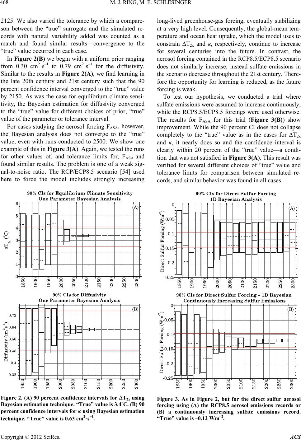 M. J. RING, M. E. SCHLESINGER 468 2125. We also varied the tolerance by which a compare- son between the “true” surrogate and the simulated re- cords with natural variability added was counted as a match and found similar results—convergence to the “true” value occurred in each case. In Figure 2(B) we begin with a uniform prior ranging from 0.30 cm2·s–1 to 0.79 cm 2·s–1 for the diffusivity. Similar to the results in Figure 2(A), we find learning in the late 20th century and 21st century such that the 90 percent confidence interval converged to the “true” value by 2150. As was the case for equilibrium climate sensi- tivity, the Bayesian estimation for diffusivity converged to the “true” value for different choices of prior, “true” value of the parameter or tolerance interval. For cases studying the aerosol forcing FASA, however, the Bayesian analysis does not converge to the “true” value, even with runs conducted to 2500. We show one example of this in Figure 3(A). Again, we tested the runs for other values of, and tolerance limits for, FASA and found similar results. The problem is one of a weak sig- nal-to-noise ratio. The RCP/ECP8.5 scenario [54] used here to force the model includes strongly increasing Figure 2. (A) 90 percent confidence intervals for T2x using Bayesian estimation technique. “True” value is 3.4˚C. (B) 90 percent confidence intervals for κ using Bayesian estimation technique. “True” value is 0.63 cm2·s−1. long-lived greenhouse-gas forcing, eventually stabilizing at a very high level. Consequently, the global-mean tem- perature and ocean heat uptake, which the model uses to constrain T2x and κ, respectively, continue to increase for several centuries into the future. In contrast, the aerosol forcing contained in the RCP8.5/ECP8.5 scenario does not similarly increase; instead sulfate emissions in the scenario decrease throughout the 21st century. There- fore the opportunity for learning is reduced, as the future forcing is weak. To test our hypothesis, we conducted a trial where sulfate emissions were assumed to increase continuously, while the RCP8.5/ECP8.5 forcings were used otherwise. The results for FASA for this trial (Figure 3(B)) show improvement. While the 90 percent CI does not collapse completely to the “true” value as in the cases for T2x and κ, it nearly does so and the confidence interval is clearly within 20 percent of the “true” value—a condi- tion that was not satisfied in Figure 3(A). This result was verified for several different choices of “true” value and tolerance limits for comparison between simulated re- cords, and similar behavior was found in all cases. Figure 3. As in Figure 2, but for the direct sulfur aerosol forcing using (A) the RCP8.5 aerosol emissions records or (B) a continuously increasing sulfate emissions record. “True” value is –0.12 Wm–2. Copyright © 2012 SciRes. ACS 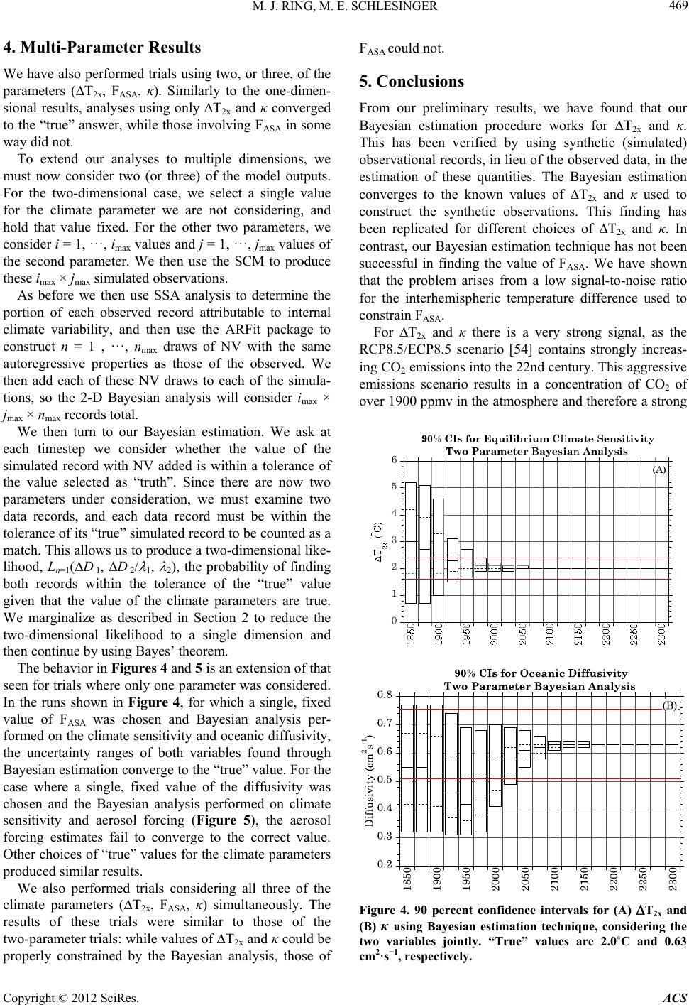 M. J. RING, M. E. SCHLESINGER 469 4. Multi-Parameter Results We have also performed trials using two, or three, of the parameters (T2x, FASA, κ). Similarly to the one-dimen- sional results, analyses using only T2x and κ converged to the “true” answer, while those involving FASA in some way did not. To extend our analyses to multiple dimensions, we must now consider two (or three) of the model outputs. For the two-dimensional case, we select a single value for the climate parameter we are not considering, and hold that value fixed. For the other two parameters, we consider i = 1, ···, imax values and j = 1, ···, jmax values of the second parameter. We then use the SCM to produce these imax × jmax simulated observations. As before we then use SSA analysis to determine the portion of each observed record attributable to internal climate variability, and then use the ARFit package to construct n = 1 , ···, nmax draws of NV with the same autoregressive properties as those of the observed. We then add each of these NV draws to each of the simula- tions, so the 2-D Bayesian analysis will consider imax × jmax × nmax records total. We then turn to our Bayesian estimation. We ask at each timestep we consider whether the value of the simulated record with NV added is within a tolerance of the value selected as “truth”. Since there are now two parameters under consideration, we must examine two data records, and each data record must be within the tolerance of its “true” simulated record to be counted as a match. This allows us to produce a two-dimensional like- lihood, Ln=1(D D , the probability of finding both records within the tolerance of the “true” value given that the value of the climate parameters are true. We marginalize as described in Section 2 to reduce the two-dimensional likelihood to a single dimension and then continue by using Bayes’ theorem. The behavior in Figures 4 and 5 is an extension of that seen for trials where only one parameter was considered. In the runs shown in Figure 4, for which a single, fixed value of FASA was chosen and Bayesian analysis per- formed on the climate sensitivity and oceanic diffusivity, the uncertainty ranges of both variables found through Bayesian estimation converge to the “true” value. For the case where a single, fixed value of the diffusivity was chosen and the Bayesian analysis performed on climate sensitivity and aerosol forcing (Figure 5), the aerosol forcing estimates fail to converge to the correct value. Other choices of “true” values for the climate parameters produced similar results. We also performed trials considering all three of the climate parameters (T2x, FASA, κ) simultaneously. The results of these trials were similar to those of the two-parameter trials: while values of T2x and κ could be properly constrained by the Bayesian analysis, those of FASA could not. 5. Conclusions From our preliminary results, we have found that our Bayesian estimation procedure works for T2x and κ. This has been verified by using synthetic (simulated) observational records, in lieu of the observed data, in the estimation of these quantities. The Bayesian estimation converges to the known values of T2x and κ used to construct the synthetic observations. This finding has been replicated for different choices of T2x and κ. In contrast, our Bayesian estimation technique has not been successful in finding the value of FASA. We have shown that the problem arises from a low signal-to-noise ratio for the interhemispheric temperature difference used to constrain FASA. For T2x and κ there is a very strong signal, as the RCP8.5/ECP8.5 scenario [54] contains strongly increas- ing CO2 emissions into the 22nd century. This aggressive emissions scenario results in a concentration of CO2 of over 1900 ppmv in the atmosphere and therefore a strong Figure 4. 90 percent confidence intervals for (A) T2x and (B) κ using Bayesian estimation technique, considering the two variables jointly. “True” values are 2.0˚C and 0.63 cm2·s−1, respectively. Copyright © 2012 SciRes. ACS 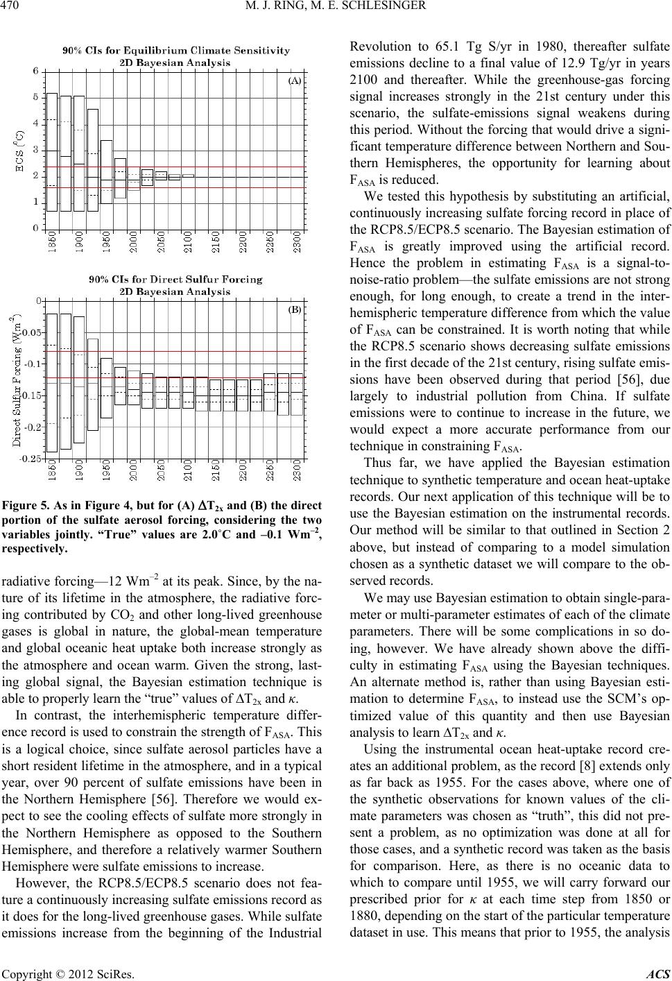 M. J. RING, M. E. SCHLESINGER 470 Figure 5. As in Figure 4, but for (A) T2x and (B) the direct portion of the sulfate aerosol forcing, considering the two variables jointly. “True” values are 2.0˚C and –0.1 Wm–2, respectively. radiative forcing—12 Wm–2 at its peak. Since, by the na- ture of its lifetime in the atmosphere, the radiative forc- ing contributed by CO2 and other long-lived greenhouse gases is global in nature, the global-mean temperature and global oceanic heat uptake both increase strongly as the atmosphere and ocean warm. Given the strong, last- ing global signal, the Bayesian estimation technique is able to properly learn the “true” values of T2x and κ. In contrast, the interhemispheric temperature differ- ence record is used to constrain the strength of FASA. This is a logical choice, since sulfate aerosol particles have a short resident lifetime in the atmosphere, and in a typical year, over 90 percent of sulfate emissions have been in the Northern Hemisphere [56]. Therefore we would ex- pect to see the cooling effects of sulfate more strongly in the Northern Hemisphere as opposed to the Southern Hemisphere, and therefore a relatively warmer Southern Hemisphere were sulfate emissions to increase. However, the RCP8.5/ECP8.5 scenario does not fea- ture a continuously increasing sulfate emissions record as it does for the long-lived greenhouse gases. While sulfate emissions increase from the beginning of the Industrial Revolution to 65.1 Tg S/yr in 1980, thereafter sulfate emissions decline to a final value of 12.9 Tg/yr in years 2100 and thereafter. While the greenhouse-gas forcing signal increases strongly in the 21st century under this scenario, the sulfate-emissions signal weakens during this period. Without the forcing that would drive a signi- ficant temperature difference between Northern and Sou- thern Hemispheres, the opportunity for learning about FASA is reduced. We tested this hypothesis by substituting an artificial, continuously increasing sulfate forcing record in place of the RCP8.5/ECP8.5 scenario. The Bayesian estimation of FASA is greatly improved using the artificial record. Hence the problem in estimating FASA is a signal-to- noise-ratio problem—the sulfate emissions are not strong enough, for long enough, to create a trend in the inter- hemispheric temperature difference from which the value of FASA can be constrained. It is worth noting that while the RCP8.5 scenario shows decreasing sulfate emissions in the first decade of the 21st century, rising sulfate emis- sions have been observed during that period [56], due largely to industrial pollution from China. If sulfate emissions were to continue to increase in the future, we would expect a more accurate performance from our technique in constraining FASA. Thus far, we have applied the Bayesian estimation technique to synthetic temperature and ocean heat-uptake records. Our next application of this technique will be to use the Bayesian estimation on the instrumental records. Our method will be similar to that outlined in Section 2 above, but instead of comparing to a model simulation chosen as a synthetic dataset we will compare to the ob- served records. We may use Bayesian estimation to obtain single-para- meter or multi-parameter estimates of each of the climate parameters. There will be some complications in so do- ing, however. We have already shown above the diffi- culty in estimating FASA using the Bayesian techniques. An alternate method is, rather than using Bayesian esti- mation to determine FASA, to instead use the SCM’s op- timized value of this quantity and then use Bayesian analysis to learn T2x and κ. Using the instrumental ocean heat-uptake record cre- ates an additional problem, as the record [8] extends only as far back as 1955. For the cases above, where one of the synthetic observations for known values of the cli- mate parameters was chosen as “truth”, this did not pre- sent a problem, as no optimization was done at all for those cases, and a synthetic record was taken as the basis for comparison. Here, as there is no oceanic data to which to compare until 1955, we will carry forward our prescribed prior for κ at each time step from 1850 or 1880, depending on the start of the particular temperature dataset in use. This means that prior to 1955, the analysis Copyright © 2012 SciRes. ACS 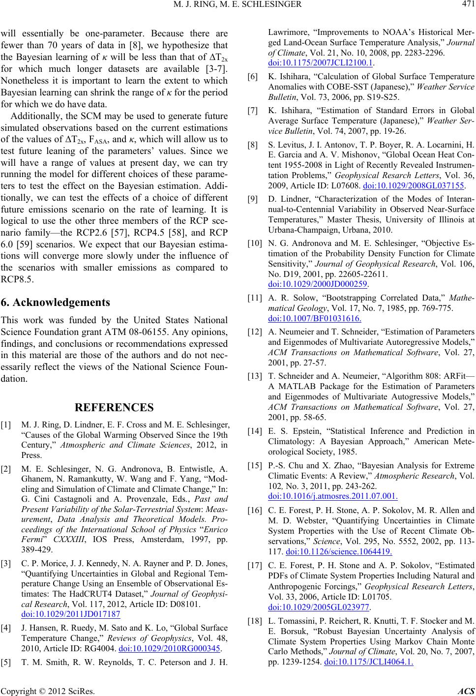 M. J. RING, M. E. SCHLESINGER 471 will essentially be one-parameter. Because there are fewer than 70 years of data in [8], we hypothesize that the Bayesian learning of κ will be less than that of T2x for which much longer datasets are available [3-7]. Nonetheless it is important to learn the extent to which Bayesian learning can shrink the range of κ for the period for which we do have data. Additionally, the SCM may be used to generate future simulated observations based on the current estimations of the values of T2x, FASA, and κ, which will allow us to test future leaning of the parameters’ values. Since we will have a range of values at present day, we can try running the model for different choices of these parame- ters to test the effect on the Bayesian estimation. Addi- tionally, we can test the effects of a choice of different future emissions scenario on the rate of learning. It is logical to use the other three members of the RCP sce- nario family—the RCP2.6 [57], RCP4.5 [58], and RCP 6.0 [59] scenarios. We expect that our Bayesian estima- tions will converge more slowly under the influence of the scenarios with smaller emissions as compared to RCP8.5. 6. Acknowledgements This work was funded by the United States National Science Foundation grant ATM 08-06155. Any opinions, findings, and conclusions or recommendations expressed in this material are those of the authors and do not nec- essarily reflect the views of the National Science Foun- dation. REFERENCES [1] M. J. Ring, D. Lindner, E. F. Cross and M. E. Schlesinger, “Causes of the Global Warming Observed Since the 19th Century,” Atmospheric and Climate Sciences, 2012, in Press. [2] M. E. Schlesinger, N. G. Andronova, B. Entwistle, A. Ghanem, N. Ramankutty, W. Wang and F. Yang, “Mod- eling and Simulation of Climate and Climate Change,” In: G. Cini Castagnoli and A. Provenzale, Eds., Past and Present Variability of the Solar-Terrestrial System: Meas- urement, Data Analysis and Theoretical Models. Pro- ceedings of the International School of Physics “Enrico Fermi” CXXXIII, IOS Press, Amsterdam, 1997, pp. 389-429. [3] C. P. Morice, J. J. Kennedy, N. A. Rayner and P. D. Jones, “Quantifying Uncertainties in Global and Regional Tem- perature Change Using an Ensemble of Observational Es- timates: The HadCRUT4 Dataset,” Journal of Geophysi- cal Research, Vol. 117, 2012, Article ID: D08101. doi:10.1029/2011JD017187 [4] J. Hansen, R. Ruedy, M. Sato and K. Lo, “Global Surface Temperature Change,” Reviews of Geophysics, Vol. 48, 2010, Article ID: RG4004. doi:10.1029/2010RG000345. [5] T. M. Smith, R. W. Reynolds, T. C. Peterson and J. H. Lawrimore, “Improvements to NOAA’s Historical Mer- ged Land-Ocean Surface Temperature Analysis,” Journal of Climate, Vol. 21, No. 10, 2008, pp. 2283-2296. doi:10.1175/2007JCLI2100.1. [6] K. Ishihara, “Calculation of Global Surface Temperature Anomalies with COBE-SST (Japanese),” Weather Service Bulletin, Vol. 73, 2006, pp. S19-S25. [7] K. Ishihara, “Estimation of Standard Errors in Global Average Surface Temperature (Japanese),” Weather Ser- vice Bulletin, Vol. 74, 2007, pp. 19-26. [8] S. Levitus, J. I. Antonov, T. P. Boyer, R. A. Locarnini, H. E. Garcia and A. V. Mishonov, “Global Ocean Heat Con- tent 1955-2008 in Light of Recently Revealed Instrumen- tation Problems,” Geophysical Resarch Letters, Vol. 36, 2009, Article ID: L07608. doi:10.1029/2008GL037155. [9] D. Lindner, “Characterization of the Modes of Interan- nual-to-Centennial Variability in Observed Near-Surface Temperatures,” Master Thesis, University of Illinois at Urbana-Champaign, Urbana, 2010. [10] N. G. Andronova and M. E. Schlesinger, “Objective Es- timation of the Probability Density Function for Climate Sensitivity,” Journal of Geophysical Research, Vol. 106, No. D19, 2001, pp. 22605-22611. doi:10.1029/2000JD000259. [11] A. R. Solow, “Bootstrapping Correlated Data,” Mathe- matical Geology, Vol. 17, No. 7, 1985, pp. 769-775. doi:10.1007/BF01031616. [12] A. Neumeier and T. Schneider, “Estimation of Parameters and Eigenmodes of Multivariate Autoregressive Models,” ACM Transactions on Mathematical Software, Vol. 27, 2001, pp. 27-57. [13] T. Schneider and A. Neumeier, “Algorithm 808: ARFit— A MATLAB Package for the Estimation of Parameters and Eigenmodes of Multivariate Autogressive Models,” ACM Transactions on Mathematical Software, Vol. 27, 2001, pp. 58-65. [14] E. S. Epstein, “Statistical Inference and Prediction in Climatology: A Bayesian Approach,” American Mete- orological Society, 1985. [15] P.-S. Chu and X. Zhao, “Bayesian Analysis for Extreme Climatic Events: A Review,” Atmospheric Research, Vol. 102, No. 3, 2011, pp. 243-262. doi:10.1016/j.atmosres.2011.07.001. [16] C. E. Forest, P. H. Stone, A. P. Sokolov, M. R. Allen and M. D. Webster, “Quantifying Uncertainties in Climate System Properties with the Use of Recent Climate Ob- servations,” Science, Vol. 295, No. 5552, 2002, pp. 113- 117. doi:10.1126/science.1064419. [17] C. E. Forest, P. H. Stone and A. P. Sokolov, “Estimated PDFs of Climate System Properties Including Natural and Anthropogenic Forcings,” Geophysical Research Letters, Vol. 33, 2006, Article ID: L01705. doi:10.1029/2005GL023977. [18] L. Tomassini, P. Reichert, R. Knutti, T. F. Stocker and M. E. Borsuk, “Robust Bayesian Uncertainty Analysis of Climate System Properties Using Markov Chain Monte Carlo Methods,” Journal of Climate, Vol. 20, No. 7, 2007, pp. 1239-1254. doi:10.1175/JCLI4064.1. Copyright © 2012 SciRes. ACS  M. J. RING, M. E. SCHLESINGER 472 [19] C. E. Forest, P. H. Stone and A. P. Sokolov, “Constrain- ing Climate Model Parameters from Observed 20th Cen- tury Changes,” Tellus A, Vol. 60, No. 5, 2008, pp. 911- 920. doi:10.1111/j.1600-0870.2008.00346.x. [20] J. D. Annan and J. C. Hargraves, “On the Generation and Interpretation of Probabilistic Estimates of Climate Sensi- tivity,” Climatic Change, Vol. 104, No. 3-4, 2011, pp. 423-436. doi:10.1007/s10584-009-9715-y. [21] S. S. Leroy, “Detecting Climate Signals: Some Bayesian Aspects,” Journal of Climate, Vol. 11, No. 4, 1998, pp. 640-651. doi:10.1175/1520-0442(1998)011<0640:DCSSBA>2.0.C O;2. [22] T. C. K. Lee, F. W. Zwiers, G. C. Hegerl, X. Zhang and M. Tsao, “A Bayesian Climate Change Detection and At- tribution Assessment,” Journal of Climate, Vol. 18, No. 13, 2006, pp. 2429-2440. doi:10.1175/JCLI3402.1. [23] S. S. Leroy and J. G. Anderson, “Optimal Detection of Regional Trends Using Global Data,” Journal of Climate, Vol. 23, No. 16, 2010, pp. 4438-4446. doi:10.1175/2010JCLI3550.1. [24] L. Tomassini, R. Knutti, G.-K. Plattner, D. P. van Vuuren, T. F. Stocker, R. B. Howarth and M. E. Borsuk, “Uncer- tainty and Risk in Climate Projections for the 21st Cen- tury: Comparing Mitigation to Non-Intervention Scenar- ios,” Climatic Change, Vol. 103, No. 3-4, 2010, pp. 399- 422. doi:10.1007/s10584-009-9763-3. [25] S.-K. Min and A. Hense, “A Bayesian Assessment of Climate Change Using Multi-Model Ensembles. Part I: Global Mean Surface Temperature,” Journal of Climate, Vol. 19, No. 13, 2006, pp. 3237-3256. doi:10.1175/JCLI3784.1. [26] S.-K. Min, D. Simonis and A. Hense, “Probabilistic Cli- mate Change Predictions Applying Bayesian Model Av- eraging,” Philosophical Transactions of the Royal Society A, Vol. 365, No. 1857, 2007, pp. 2103-2116. doi:10.1098/rsta.2007.2070. [27] R. L. Smith, C. Tebaldi, D. Nychka and L. O. Mearns, “Bayesian Modeling of Uncertainty in Ensembles of Cli- mate Models,” Journal of the American Statistical Asso- ciation, Vol. 104, No. 485, 2009, pp. 97-116. doi:10.1198/jasa.2009.0007. [28] R. Furrer, R. Knutti, S. R. Sain, D. W. Nychka and G. A. Meehl, “Spatial Patterns of Probabilistic Temperature Change Projections from a Multivariate Bayesian Analy- sis,” Geophysical Research Letters, Vol. 34, 2006, Article ID: L06711. doi:10.1029/2006GL027754. [29] R. Furrer, S. R. Sain, D. Nychka and G. A. Meehl, “Mul- tivariate Bayesian Analysis of Atmosphere-Ocean Gen- eral Circulation Models,” Environmental and Ecological Statistics, Vol. 14, No. 3, 2007, pp. 249-266. doi:10.1007/s10651-007-0018-z. [30] C. Tebaldi and B. Sanso, “Joint Projections of Tempera- ture and Precipitation Change from Multiple Climate Models: A Hierarchical Bayesian Approach,” Journal of the Royal Statistical Society A, Vol. 172, No. 1, 2009, pp. 83-106. doi:10.1111/j.1467-985X.2008.00545.x. [31] F. Beltran, B. Sanso, R. Lemos and R. Mendelssohn, “Joint Projections of North Pacific Sea Surface Tempera- ture from Different Global Climate Models,” University of California, Santa Cruz, 2011. [32] C. Tebaldi, L. O. Mearns, D. Nychka and R. W. Smith, “Regional Probabilities of Precipitation Change: A Bay- esian Analysis of Multimodel Simulations,” Geophysical Research Letters, Vol. 31, 2004, Article ID: L24213. [33] C. Tebaldi, R. W. Smith, D. Nychka and L. O. Mearns, “Quantifying Uncertainty in Projections of Regional Cli- mate Change: A Bayesian Approach to the Analysis of Multimodel Ensembles,” Journal of Climate, Vol. 18, No. 10, 2005, pp. 1524-1540. doi:10.1175/JCLI3363.1. [34] S.-K. Min and A. Hense, “A Bayesian Assessment of Climate Change Using Multi-Model Ensembles. Part II: Regional and Seasonal Mean Surface Temepratures,” Journal of Climate, Vol. 20, No. 12, 2007, pp. 2769-2790. doi:10.1175/JCLI4178.1. [35] J. B. Elsner and B. H. Bossak, “Bayesian Analysis of US Hurricane Climate,” Journal of Climate, Vol. 14, No. 23, 2001, pp. 4341-4350. doi:10.1175/1520-0442(2001)014<4341:BAOUSH>2.0.C O;2. [36] P.-S. Chu and X. Zhao, “Bayesian Change-Point Analysis of Tropical Cyclone Activity: The Central North Pacific case,” Journal of Climate, Vol. 17, No. 24, 2004, pp. 4893-4901. doi: 10.1175/JCLI-3248.1. [37] J. B. Elsner and T. H. Jagger, “Prediction Models for Annual US Hurricane Counts,” Journal of Climate, Vol. 19, No. 12, 2006, pp. 2935-2952. doi:10.1175/JCLI3729.1. [38] X. Zhao and P.-S. Chu, “Bayesian Multiple Changepoint Analysis of Hurricane Activity in the Eastern North Pa- cific: A Markov Chain Monte Carlo Approach,” Journal of Climate, Vol. 19, No. 4, 2006, pp. 564-578. doi:10.1175/JCLI3628.1. [39] S. J. Camargo, A. W. Robertson, S. J. Gaffney, P. Smyth and M. Ghil, “Cluster Analysis of Typhoon Tracks. Part I: General Properties,” Journal of Climate, Vol. 20, No. 14, 2007, pp. 3635-3653. doi:10.1175/JCLI4188.1. [40] P.-S. Chu and X. Zhao, “A Bayesian Regression Ap- proach for Predicting Seasonal Tropical Cyclone Activity over the Central North Pacific,” Journal of Climate, Vol. 20, No. 15, 2007, pp. 4002-4013. doi:10.1175/JCLI4214.1. [41] C.-H. Ho, H. S. Kim, P.-S. Chu and J.-H. Kim, “Seasonal Prediction of Tropical Cyclone Frequency over the East China Sea through a Bayesian Poisson-Regression Me- thod,” Asia-Pacific Journal of Atmospheric Sciences, Vol. 45, No. 1, 2009, pp. 45-54. [42] J.-Y. Tu, C. Chou and P.-S. Chu, “The Abrupt Shift of Typhoon Activity in the Vicinity of Taiwan and Its Asso- ciation with Western North Pacific-East Asian Climate Change,” Journal of Climate, Vol. 22, No. 13, 2009, pp. 3617-3628. doi:10.1175/2009JCLI2411.1. [43] S. S. Chand, K. J. E. Walsh and J. C. L. Chan, “A Bayes- ian Regression Approach to Seasonal Prediction of Tropi- cal Cyclones Affecting the Fiji Region,” Journal of Cli- mate, Vol. 23, No. 13, 2010, pp. 3425-3445. doi:10.1175/2010JCLI3521.1. [44] P.-S. Chu, X. Zhao, C.-H. Ho, H.-S. Kim, M.-M. Lu and Copyright © 2012 SciRes. ACS  M. J. RING, M. E. SCHLESINGER Copyright © 2012 SciRes. ACS 473 J.-H. Kim, “Bayesian Forecasting of Seasonal Typhoon Activity: A Track Pattern-Oriented Categorization Ap- proach,” Journal of Climate, Vol. 23, No. 24, 2010, pp. 6654-6668. doi:10.1175/2010JCLI3710.1. [45] T. H. Jagger and J. B. Elsner, “A Consensus Model for Seasonal Hurricane Prediction,” Journal of Climate, Vol. 23, No. 22, 2009, pp. 6090-6099. doi:10.1175/2010JCLI3686.1. [46] M.-M. Lu, P.-S. Chu and Y.-C. Lin, “Seasonal Prediction of Tropical Cyclone Activity in the Vicinty of Taiwan Using the Bayesian Multivariate Regression Method,” Weather and Forecasting, Vol. 25, No. 6, 2010, pp. 1780- 1795. doi:10.1175/2010WAF2222408.1. [47] M. Kallache, E. Maksimovich, P.-A. Michelangeli and P. Naveau, “Multi-Model Combination by a Bayesian Hier- archical Model: Assessment of Ice Accumulation over the Oceanic Arctic Region,” Journal of Climate, Vol. 23, No. 20, 2010, pp. 5421-5436. doi:10.1175/2010JCLI3107.1. [48] B. F. Hobbs, “Bayesian Methods for Analysing Climate Change and Water Resource Uncertainties,” Journal of Environmental Management, Vol. 49, No. 1, 1997, pp. 53-72. doi:10.1006/jema.1996.0116, [49] L. Perreault, J. Bernier, B. Bobee and E. Parent, “Bayes- ian Change-Point Analysis in Hydrometeorological Time Series. Part 1: The Normal Model Revisited,” Journal of Hydrology, Vol. 235, No. 3-4, 2000, pp. 221-241. doi:10.1016/S0022-1694(00)00270-5. [50] L. Perreault, J. Bernier, B. Bobee and E. Parent, “Bayes- ian Change-Point Analysis in Hydrometeorological Time Series. Part 2: Comparison of Change-Point Models and Forecasting,” Journal of Hydrology, Vol. 235, No. 3-4, 2000, pp. 242-263. doi:10.1016/S0022-1694(00)00271-7. [51] B. Renard, M. Land and P. Bois, “Statistical Analysis of Extreme Events in A Non-Stationary Context via a Bayesian Framework: Case Study with Peak-over-Thre- shold Data,” Stochastic Environmental Research and Risk Assessment, Vol. 21, No. 2, 2006, pp. 97-112. doi:10.1007/s00477-006-0047-4. [52] C. H. R. Lima and U. Lall, “Spatial Scaling in a Changing Climate: A Hierarchical Bayesian Model for Non-Sta- tionary Multi-Site Annual Maximum and Monthly Stream- flow,” Journal of Hydrology, Vol. 383, No. 3-4, 2010, pp. 307-318. doi:10.1016/j.jhydrol.2009.12.045. [53] D. Peavoy and C. Franzke, “Bayesian Analysis of Rapid Climate Change during the Last Glacial Using Greenland Delta O-18 Data,” Climate of the Past, Vol. 6, No. 6, pp. 787-794. doi:10.5194/cp-6-787-2010. [54] K. Riahi, et al., “RCP8.5—A Scenario of Comparatively High Greenhouse Emissions,” Climatic Change, Vol. 109, No. 1-2, 2011, pp. 33-57. doi:10.1007/s10584-011-0149-y. [55] M. Ghil, M. R. Allen, M. D. Dettinger, K. Ide, D. Kondrashov, M. E. Mann, A. W. Robertson, A. Saunders, Y. Tian, F. Varadi and P. Yiou, “Advanced Spectral Methods for Climatic Time Series,” Reviews of Geophys- ics, Vol. 40, No. 1, 2002, Article ID: 1003. doi:10.1029/2000RG000092. [56] S. J. Smith, J. van Aardenne, Z. Klimont, R. Andres, A. C. Volke and S. Delgado Arias, “Anthropogenic Sulfur Di- oxide Emissions 1850-2005,” Atmospheric Chemistry and Physics, Vol. 11, 2011, pp. 1101-1116. doi:10.5194/acp-11-1101-2011. [57] D. P. van Vurren, et al., “RCP2.6: Exploring the Possibil- ity to Keep Global Mean Temperature Increase below 2˚C,” Climatic Change, Vol. 109, No. 1-2, 2011, pp. 95- 116. doi:10.1007/s10584-011-0152-3. [58] A. M. Thomson, et al., “RCP4.5: A Pathway for Stabili- zation of Radiative Forcing by 2100,” Climatic Change, Vol. 109, No. 1-2, 2011, pp. 77-94. doi:10.1007/s10584-011-0151-4. [59] T. Masui, et al., “An Emission Pathway for Stabilization at 6 Wm−2 Radiative Forcing,” Climatic Change, Vol. 109, No. 1-2, 2011, pp. 59-76. doi:10.1007/s10584-011-0150-5.
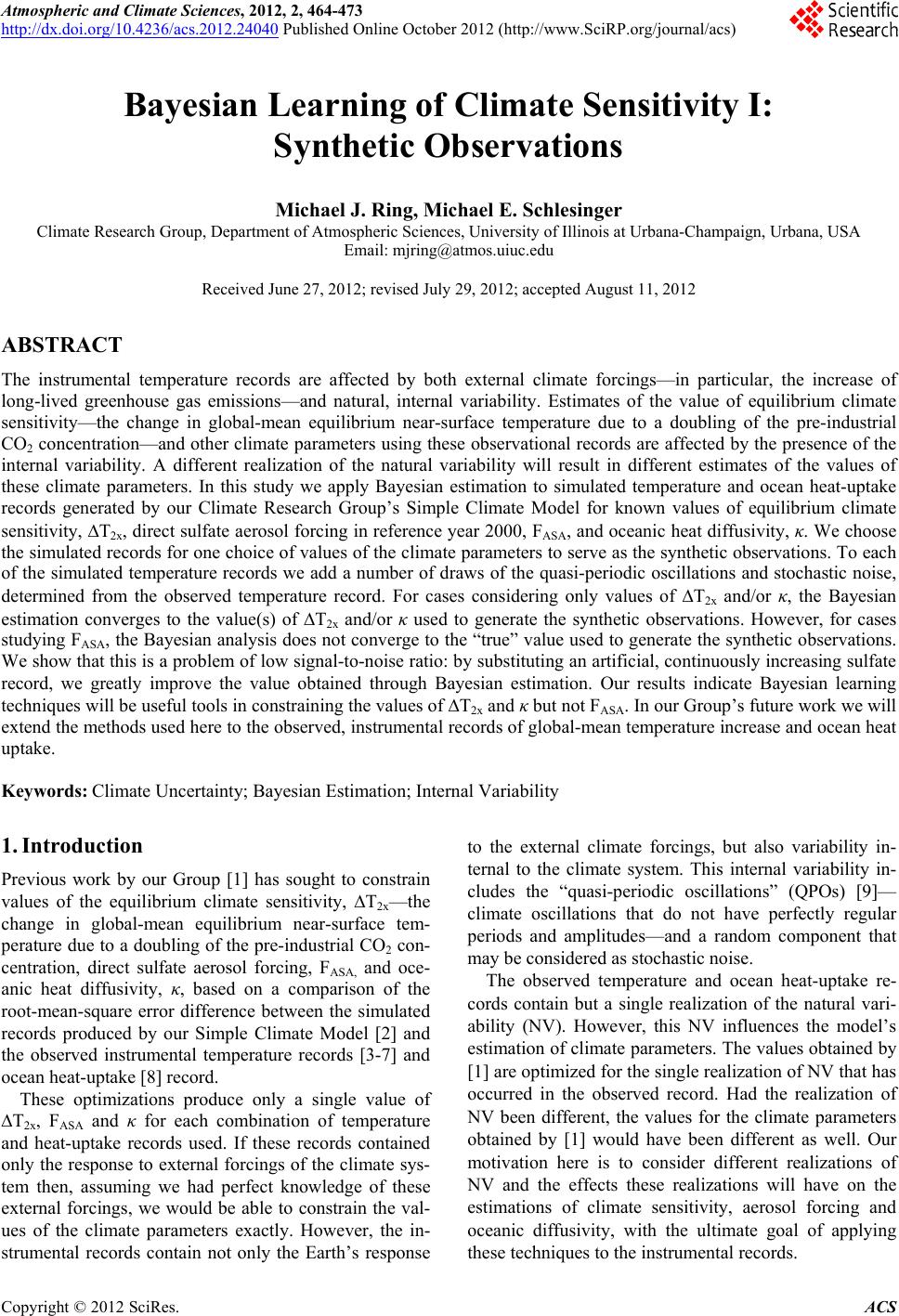
|