Applied Mathematics, 2012, 3, 1448-1462
http://dx.doi.org/10.4236/am.2012.330204 Published Online October 2012 (http://www.SciRP.org/journal/am)
Comparison of Alternative Strategies for Multilevel
Optimization of Hierarchical Systems
Saber DorMohammadi, Masoud Rais-Rohani
Center for Advanced Vehicular Systems, Mississippi State University, Starkville, USA
Received July 10, 2012; revised August 10, 2012; accepted August 17, 2012
ABSTRACT
The augmented Lagrangian penalty formulation and four different coordination strategies are used to examine the nu-
merical behavior of Analytical Target Cascading (ATC) for multilevel optimization of hierarchical systems. The coor-
dination strategies considered include augmented Lagrangian using the method of multipliers and alternating direction
method of multipliers, diagonal quadratic approximation, and truncated diagonal quadratic approximation. Properties
examined include computational cost and solution accuracy based on the selected values for the different parameters
that appear in each formulation. The different strategies are implemented using two- and three-level decomposed exam-
ple problems. While the results show the interaction between the selected ATC formulation and the values of associated
parameters, they clearly highlight the impact they could have on both the solution accuracy and computational cost.
Keywords: Analytical Target Cascading; Multilevel Design Optimization; Augmented Lagrangian;
Method of Multipliers
1. Introduction
A complex optimization problem may be decomposed
into two or more subsystems with partitioned design
variables and separate objective functions and design
constraints. The layered architecture of hierarchically
decomposed multilevel systems is illustrated by the ex-
ample in Figure 1; the hierarchy can be expanded to in-
clude several levels with each containing multiple ele-
ments. Because the number of design variables in each
element represents a fraction of the total set, dimension-
ality of each element optimization problem is reduced.
Decomposed optimization problems require a coordina-
tion strategy that in the ensuing iterative solution process
ensures satisfaction of system-level design criteria and
proper convergence to an optimum design.
Analytical target cascading (ATC) [1,2] was devel-
oped for systems such as that shown in Figure 1. In the
initial formulation of ATC [2-5], deviation tolerances
Element 34
Element 11
Element 23
Element 22
Element 35 Element 36
Figure 1. An illustrative model of a hierarchically decom-
posed multilevel system.
were defined for the responses and targets as well as the
linking (or shared design) variables. The multilevel op-
timization problem was solved while minimizing the
deviation tolerances and satisfying the design constraints.
ATC solution has been shown to converge to a point
that satisfies the necessary optimality conditions of the
original design optimization problem [6]. Using a for-
mulation of ATC with similarities to that in [3], the ine-
quality constraints on deviation tolerances were brought
into the objective function to form an augmented objec-
tive function; this formulation included the addition of
weight factors to the deviation tolerances.
The scaled tolerance formulation [3] was used in [7] to
investigate the numerical behavior of the ATC method-
ology and the local convergence properties of different
coordination strategies. They examined the effects of
linking variables, subproblem solution accuracy, and the
number of significant digits on numerical stability.
The commonly used ATC formulations are based on
quadratic penalty (QP) functions [7-10]. Numerical ex-
periments with these formulations show significant
computational effort to obtain accurate solutions. The QP
functions minimize the consistency constraints (equality
or inequality) to force targets and responses to match.
Ideally, these consistency constraints have to be relaxed,
allowing inconsistencies between targets and responses
that are gradually eliminated in the iterative solution
process. For the QP function, in general, large weight
C
opyright © 2012 SciRes. AM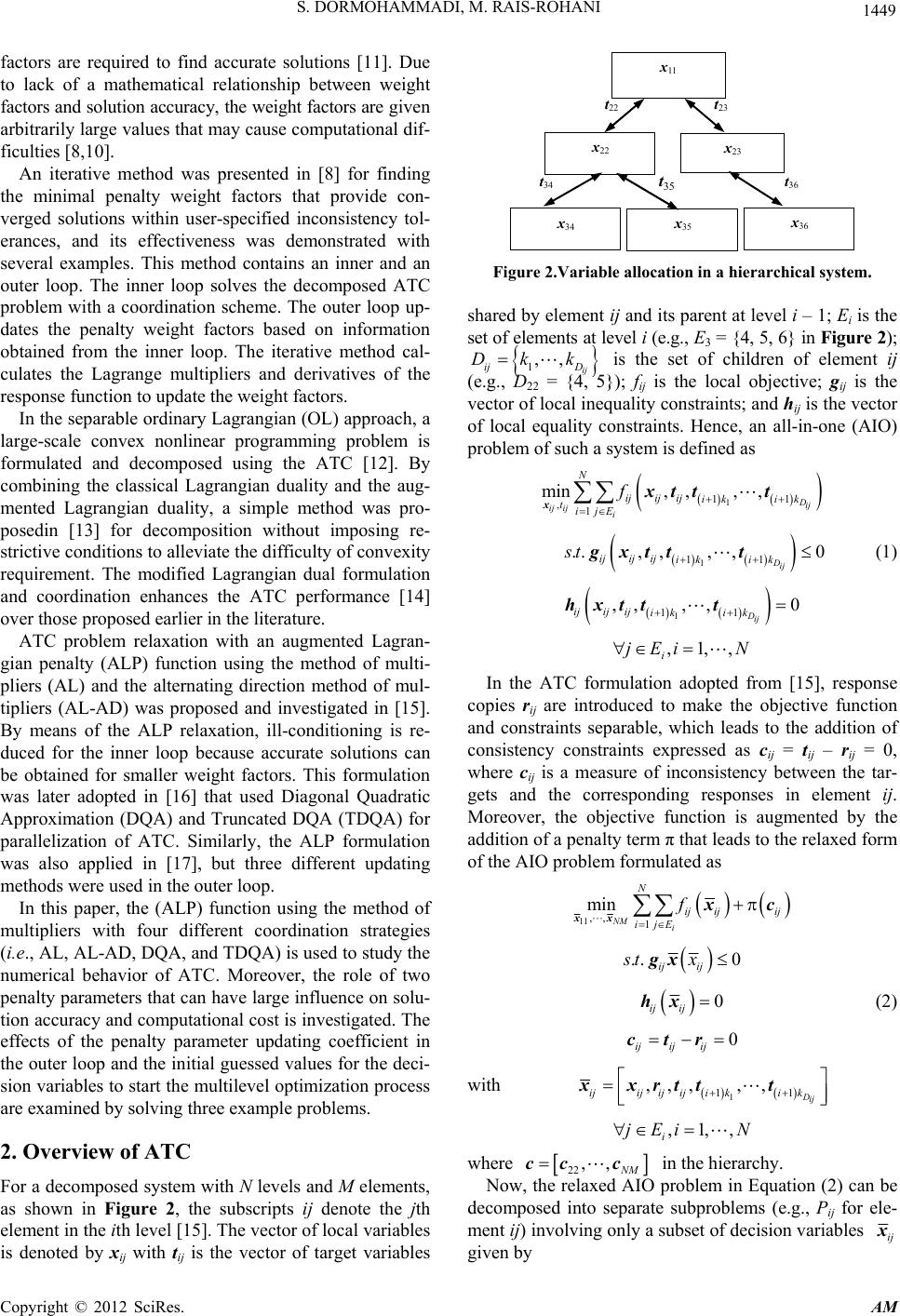

S. DORMOHAMMADI, M. RAIS-ROHANI 1449
factors are required to find accurate solutions [11]. Due
to lack of a mathematical relationship between weight
factors and solution accuracy, the weight factors are given
arbitrarily large values that may cause computational dif-
ficulties [8,10].
An iterative method was presented in [8] for finding
the minimal penalty weight factors that provide con-
verged solutions within user-specified inconsistency tol-
erances, and its effectiveness was demonstrated with
several examples. This method contains an inner and an
outer loop. The inner loop solves the decomposed ATC
problem with a coordination scheme. The outer loop up-
dates the penalty weight factors based on information
obtained from the inner loop. The iterative method cal-
culates the Lagrange multipliers and derivatives of the
response function to update the weight factors.
In the separable ordinary Lagrangian (OL) approach, a
large-scale convex nonlinear programming problem is
formulated and decomposed using the ATC [12]. By
combining the classical Lagrangian duality and the aug-
mented Lagrangian duality, a simple method was pro-
posedin [13] for decomposition without imposing re-
strictive conditions to alleviate the difficulty of convexity
requirement. The modified Lagrangian dual formulation
and coordination enhances the ATC performance [14]
over those proposed earlier in the literature.
ATC problem relaxation with an augmented Lagran-
gian penalty (ALP) function using the method of multi-
pliers (AL) and the alternating direction method of mul-
tipliers (AL-AD) was proposed and investigated in [15].
By means of the ALP relaxation, ill-conditioning is re-
duced for the inner loop because accurate solutions can
be obtained for smaller weight factors. This formulation
was later adopted in [16] that used Diagonal Quadratic
Approximation (DQA) and Truncated DQA (TDQA) for
parallelization of ATC. Similarly, the ALP formulation
was also applied in [17], but three different updating
methods were used in the outer loop.
In this paper, the (ALP) function using the method of
multipliers with four different coordination strategies
(i.e., AL, AL-AD, DQA, and TDQA) is used to study the
numerical behavior of ATC. Moreover, the role of two
penalty parameters that can have large influence on solu-
tion accuracy and computational cost is investigated. The
effects of the penalty parameter updating coefficient in
the outer loop and the initial guessed values for the deci-
sion variables to start the multilevel optimization process
are examined by solving three example problems.
2. Overview of ATC
For a decomposed system with N levels and M elements,
as shown in Figure 2, the subscripts ij denote the jth
element in the ith level [15]. The vector of local variables
is denoted by xij with tij is the vector of target variables
t
23
t
22
t
34
t
35
t
36
x
34
x
11
x
23
x
22
x
35
x
36
Figure 2.Variable allocation in a hierarchical system.
shared by element ij and its parent at level i – 1; Ei is the
set of lements at level i (e.g., E3 = {4, 5, 6} in Figure 2); e

 1,,Dk k
ij
ijD is the set of children of element ij
(e.g., D22 = {4, 5}); fij is the local objective; gij is the
vector of local inequality constraints; and hij is the vector
of local equality constraints. Hence, an all-in-one (AIO)
problem of such a system is defined as
 


1
11
,1
min, ,,,
xxttt Dij
ij iji
N
ijij ijik ik
tjEi
f

 
 


1
11
.., ,,,0
Dij
ijij ijik ik
st  gxtt t (1)
 


1
11
,,, ,0hxttt Dij
ijij ijik ik

,1,,
i
jEi N


In the ATC formulation adopted from [15], response
copies rij are introduced to make the objective function
and constraints separable, which leads to the addition of
consistency constraints expressed as cij = tij – rij = 0,
where cij is a measure of inconsistency between the tar-
gets and the corresponding responses in element ij.
Moreover, the objective function is augmented by the
addition of a penalty term π that leads to the relaxed form
of the AIO problem formulated as
 
11 ,, 1
min
xx xc
Mi N
N
ij iji
i
j
jE
f





.. 0
ij ij
stx gx


0hx
ijij (2)
0ctr
ijij ij


with
 
1
11
,,,, ,xrtt txDij
ijij ij ijikik








,1,,
i
jEi N


where


22 ,,cc c NM
 in the hierarchy.
Now, the relaxed AIO problem in Equation (2) can be
decomposed into separate subproblems (e.g., Pij for ele-
ment ij) involving only a subset of decision variables xij
given by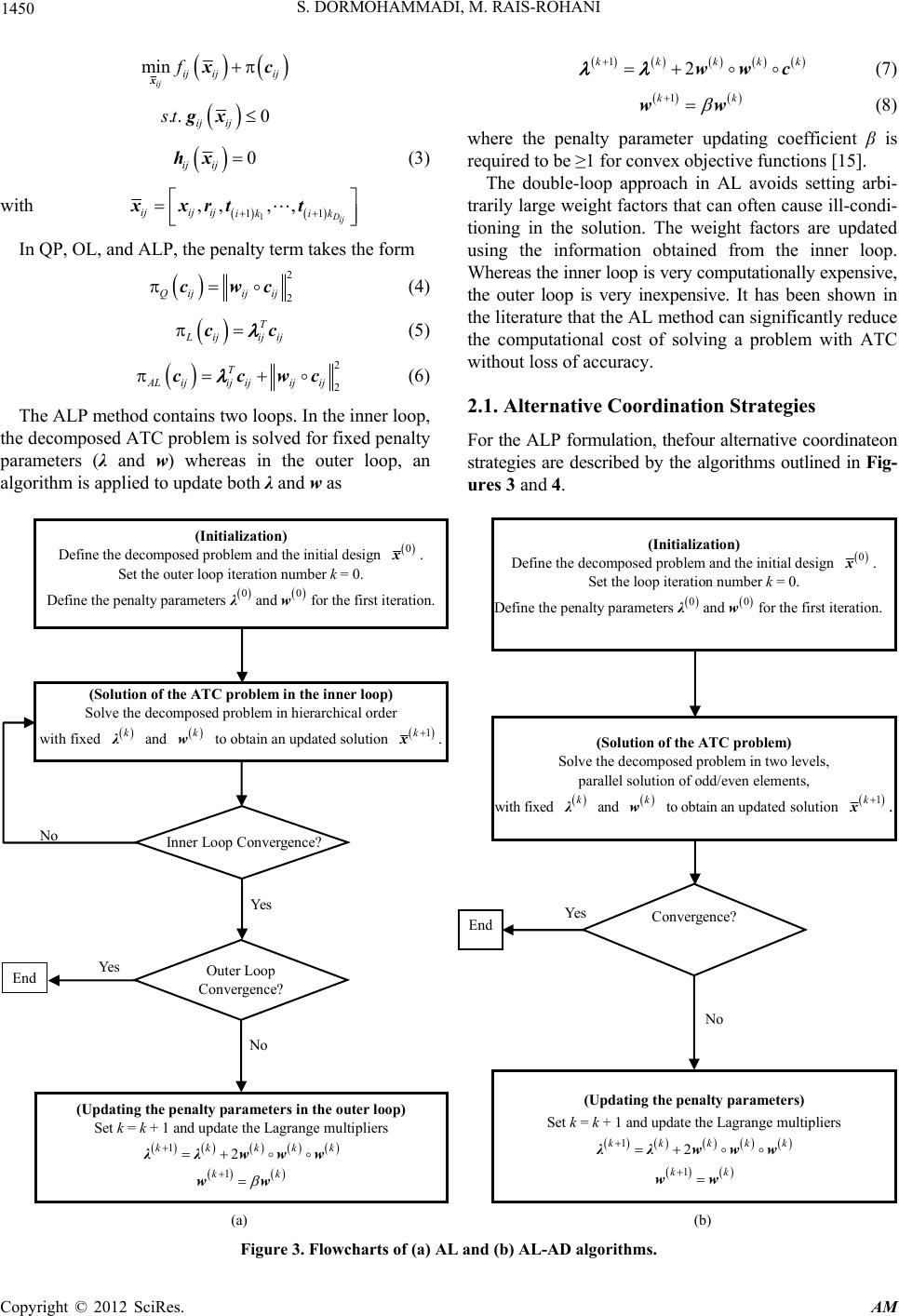

S. DORMOHAMMADI, M. RAIS-ROHANI
1450
 
min
xcx
ij
ij ijij
f
 
12wwc

kkkk k
k
(7)
  1
ww
k

 (8)

.. 0xgij ij st 
where the penalty parameter updating coefficient β is
required to be ≥1 for convex objective functions [15].

0hx
ij ij

(3)
with
 
1
11
,,, ,xrt txDij
ijij ijik ik







The double-loop approach in AL avoids setting arbi-
trarily large weight factors that can often cause ill-condi-
tioning in the solution. The weight factors are updated
using the information obtained from the inner loop.
Whereas the inner loop is very computationally expensive,
the outer loop is very inexpensive. It has been shown in
the literature that the AL method can significantly reduce
the computational cost of solving a problem with ATC
without loss of accuracy.
In QP, OL, and ALP, the penalty term takes the form

2
2
cwc
Qijij ij
 (4)

c 
Tc
L
ijij ij
 (5)

2
2
ccwc 
T
ALijij ijijij
 (6)
2.1. Alternative Coordination Strategies
The ALP method contains two loops. In the inner loop,
the decomposed ATC problem is solved for fixed penalty
parameters (λ and w) whereas in the outer loop, an
algorithm is applied to update both λ and w as
For the ALP formulation, thefour alternative coordinateon
strategies are described by the algorithms outlined in Fig-
ures 3 and 4.
(Initialization)
Define the decomposed problem and the initial design

0
x .
Set the loop iteration number k = 0.
Define the penalty parameters

0
λ
and

0
w
for the first iteration.
(Solution of the ATC problem)
Solve the decomposed problem in two levels,
parallel solution of odd/even elements,
with fixed

λ
k
and

wk to obtain an updated solution

1
xk

.
End
(Updating the pe nalty parameters)
Set k = k + 1 and update the Lagrange multipliers
 
12λλwww kkkkk 
 
1
ww
kk
No
YesConvergence?
(Initialization)
Define the decomposed problem and the initial design

0
x .
Set the outer loop iteration number k = 0.
Define the penalty parameters

0
λ
and

0
w for the first iteration.
(Solution of the ATC problem in the inner loop)
Solve the decomposed problem in hierarchical order
with fixed

λ
k
and

wk to obtain an updated solution
 1
xk

.
No
Yes
End
(Updating the penalty parameters in the outer loop)
Set k = k + 1 and update the Lagrange multipliers
  
12λλwww kkkkk 
 
1
ww
kk


Yes
No
Outer Loop
Convergence?
Inner Loop Convergence?
(a) (b)
Figure 3. Flowcharts of (a) AL and (b) AL-AD algorithms.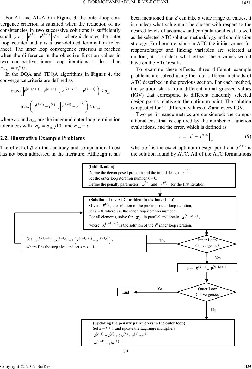

S. DORMOHAMMADI, M. RAIS-ROHANI 1451
For AL and AL-AD in Figure 3, the outer-loop con-
vergence criterion is satisfied when the reduction of in-
consistencies in two successive solutions is sufficiently
small (i.e.,
 
1
cc
kk


, where k denotes the outer
loop counter and τ is a user-defined termination toler-
ance). The inner loop convergence criterion is reached
when the difference in the objective function values in
two consecutive inner loop iterations is less than
10
ATC

 .
In the DQA and TDQA algorithms in Figure 4, the
convergence criteria are defined as


1, 11,1, 11,
max ,ttrr
ksks ksks
in
σ
 



 
11
max ,ttrr
k
kkk
out
σ
 







where σin and σout are the inner and outer loop termination
tolerances with 10
in out
σσ and σout = τ.
2.2. Illustrative Example Problems
The effect of β on the accuracy and computational cost
has not been addressed in the literature. Although it has
been mentioned that β can take a wide range of values, it
is unclear what value must be chosen with respect to the
desired levels of accuracy and computational cost as well
as the selected ATC solution methodology and coordination
strategy. Furthermore, since in ATC the initial values for
response/target and linking variables are selected at
random, it is unclear what effects these values would
have on the ATC results.
To examine these effects, three different example
problems are solved using the four different methods of
ATC described in the previous section. For each method,
the solution starts from different initial guessed values
(IGV) that correspond to different randomly selected
design points relative to the optimum point. The solution
is repeated for 20 different values of β and every IGV.
Two performance metrics are considered: the compu-
tational cost that is captured by the number of function
evaluations, and the error, which is defined as
*ATC
xxe  (9)
where x* is the exact optimum design point and xATC is
the solution found by ATC. All of the ATC formulations
Yes
End
(Updating the penalty parameters in the outer loop)
Set k = k + 1 and update the Lagrange multipliers









12
λ
λ
wwc
kkkkk





1
ww
kk


No
Set
 



1, 11,1, 11,
Γxx xx
ksksks ks 
 
,
where Γ is the step size, and set s = s + 1.
Set
 
11,1
xx
kks

No
Yes
Inner Loop
Convergence?
(Solution of the ATC proble m in the inner loop)
Given

xk , the solution of the previous outer loop iteration,
set s = 0, where s is the inner loop iteration number.
For all elements, solve for
xij
in parallel and obtain


1, 1
xks


,
where


1, 1
xks


is the solution of the s
th
inner loop iteration.
Outer Loop
Convergence?
(Initial iza tio n)
Define the decomposed problem and the initial design

0
x .
Set the outer loop iteration number k = 0.
Define the penalty parameters

0
λ
and

0
w for the first iteration.
(a)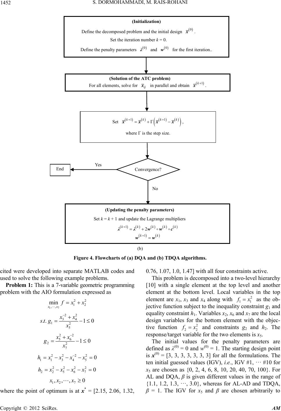

S. DORMOHAMMADI, M. RAIS-ROHANI
1452
(Initial iza tio n)
Define the decomposed problem and the initial design

0
x .
Set the iteration number k = 0.
Define the penalty parameters

0
λ
and

0
w for the first iteration..
(Solut ion of the ATC proble m)
For all elements, solve for xij in parallel and obtain
 1
xk

.
Convergence?
(Updating the penalty parameters)
Set k = k + 1 and update the Lagrange multipliers
 
12λλwwc kkkkk 




1
ww
kk
N
o
Yes
End
Set
   


11
Γxx xx
kk kk
  ,
where Γ is the step size.
(b)
Figure 4. Flowcharts of (a) DQA and (b) TDQA algorithms.
cited were developed into separate MATLAB codes and
used to solve the following example problems.
Problem 1: This is a 7-variable geometric programming
problem with the AIO formulation expressed as
17
22
12
,,
min
xx
f
xx

2
3
2
4
12
5
..1 0
xx
st gx


22
56
22
7
10
xx
gx



22 22
11 345
0hxxx x

 
2222
22567
0h xxxx
12 7
,,, 0xx x
where the point of optimum is at x* = [2.15, 2.06, 1.32,
0.76, 1.07, 1.0, 1.47] with all four constraints active.
This problem is decomposed into a two-level hierarchy
[10] with a single element at the top level and another
element at the bottom level. Local variables in the top
element are x1, x3 and x4 along with 1
2
1
f
x as the ob-
jective function subject to the inequality constraint g1 and
equality constraint h1. Variables x2, x6 and x7 are the local
design variables for the bottom element with the objec-
tive function 2
2
2
f
x

and constraints g2 and h2. The
response/target variable for the two elements is x5.
The initial values for the penalty parameters are
defined as λ(0) = 0 and w(0) = 1. The starting design point
is x(0) = [3, 3, 3, 3, 3, 3, 3] for all the formulations. The
ten initial guessed values (IGV), i.e., IGV #1, ··· #10 for
x5 are chosen as {0, 2, 4, 6, 8, 10, 20, 40, 70, 100}. For
AL and DQA, β is given different values in the range of
{1.1, 1.2, 1.3, ···, 3.0}, whereas for AL-AD and TDQA,
β = 1. The IGV for x5 and β are chosen arbitrarily to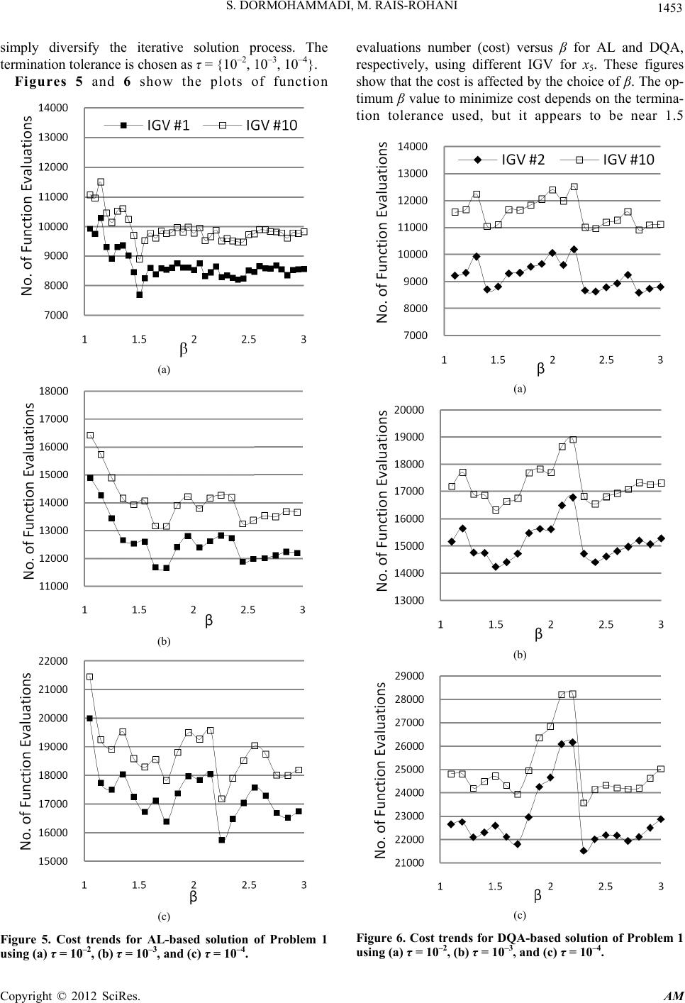

S. DORMOHAMMADI, M. RAIS-ROHANI 1453
simply diversify the iterative solution process. The
termination tolerance is chosen as τ = {10–2, 10–3, 10–4}.
Figures 5 and 6 show the plots of function
(a)
(b)
(c)
Figure 5. Cost trends for AL-based solution of Problem 1
using (a) τ = 10–2, (b) τ = 10–3, and (c) τ = 10–4.
evaluations number (cost) versus β for AL and DQA,
respectively, using different IGV for x5. These figures
show that the cost is affected by the choice of β. The op-
timum β value to minimize cost depends on the termina-
tion tolerance used, but it appears to be near 1.5
(a)
(b)
(c)
Figure 6. Cost trends for DQA-based solution of Problem 1
using (a) τ = 10–2, (b) τ = 10–3, and (c) τ = 10–4.

S. DORMOHAMMADI, M. RAIS-ROHANI
1454
or 2.3 for most cases. For different IGV, the relationship
between cost and β is similar, but it is not necessarily
monotonic. Due to this similarity, only the upper and
lower bounds are shown for each case using the corre-
sponding IGV numbers. It appears that the value of β
also has an influence on the error, especially for larger
tolerances as shown in Figure 7. The solution error
trends for different IGV are identical; hence, the plot of
error from Equation (9) versus β is shown for only one
case. Figure 8 is used to further highlight the effect of
IGV on both function evaluations and error under differ-
ent solution strategies and convergence tolerances. The
plots are shown only for β = 2 case with three conver-
gence tolerance values. The dependency of error on IGV
for AL-AD and TDQA is very high at τ = 10–2, but
minimal or nonexistent at τ = 10–3 and τ = 10–4. Thus,
TDQA and AL-AD are much more dependent on IGV
than DQA and AL. Theefficiency of AL and DQA
methods changes drastically with tighter termination tol-
erance, while solution error for AL and DQA does not
change very much. Hence, for larger τ, AL and DQA are
less costly, whereas for smaller τ, AL-AD and TDQA are
more efficient.
Problem 2: This is a 14-variable geometric program-
ming problem with the AIO formulation expressed as [5]
12 14
22
12
,,,
min
xx x
f
xx

22
34
12
5
.. 1
xx
st gx



22
56
22
7
1
xx
gx




22
89
32
11
1
xx
gx



(a)
(b)
Figure 7. Error trends for (a) AL and (b) DQA solutions of Problem 1 using x5 = 6 with τ = {10–2, 10–3, 10–4}.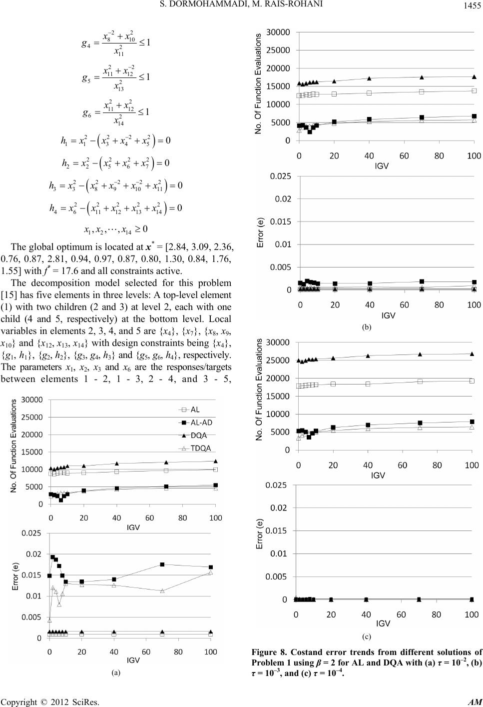

S. DORMOHAMMADI, M. RAIS-ROHANI 1455
22
810
42
11
1
xx
gx


22
11 12
52
13
1
xx
gx



22
11 12
62
14
1
xx
gx



2222
11345 0hx xxx

 

2 222
22 5670hx xxx 

22222
338910110hxxx x x

 

22222
4611 1213 140hxx x x x 
12 14
,,, 0xxx
The global optimum is located at x* = [2.84, 3.09, 2.36,
0.76, 0.87, 2.81, 0.94, 0.97, 0.87, 0.80, 1.30, 0.84, 1.76,
1.55] with f* = 17.6 and all constraints active.
The decomposition model selected for this problem
[15] has five elements in three levels: A top-level element
(1) with two children (2 and 3) at level 2, each with one
child (4 and 5, respectively) at the bottom level. Local
variables in elements 2, 3, 4, and 5 are {x4}, {x7}, {x8, x9,
x10} and {x12, x13, x14} with design constraints being {x4},
{g1, h1}, {g2, h2}, {g3, g4, h3} and {g5, g6, h4}, respectively.
The parameters x1, x2, x3 and x6 are the responses/targets
between elements 1 - 2, 1 - 3, 2 - 4, and 3 - 5,
(a)
(b)
(c)
Figure 8. Costand error trends from different solutions of
Problem 1 using β = 2 for AL and DQA with (a) τ = 10–2, (b)
τ = 10–3, and (c) τ = 10–4.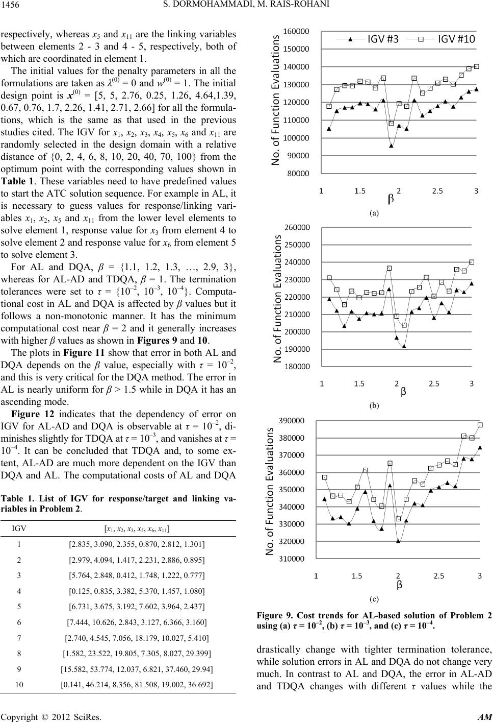

S. DORMOHAMMADI, M. RAIS-ROHANI
1456
respectively, whereas x5 and x11 are the linking variables
between elements 2 - 3 and 4 - 5, respectively, both of
which are coordinated in element 1.
The initial values for the penalty parameters in all the
formulations are taken as λ(0) = 0 and w(0) = 1. The initial
design point is x(0) = [5, 5, 2.76, 0.25, 1.26, 4.64,1.39,
0.67, 0.76, 1.7, 2.26, 1.41, 2.71, 2.66] for all the formula-
tions, which is the same as that used in the previous
studies cited. The IGV for x1, x2, x3, x4, x5, x6 and x11 are
randomly selected in the design domain with a relative
distance of {0, 2, 4, 6, 8, 10, 20, 40, 70, 100} from the
optimum point with the corresponding values shown in
Table 1. These variables need to have predefined values
to start the ATC solution sequence. For example in AL, it
is necessary to guess values for response/linking vari-
ables x1, x2, x5 and x
11 from the lower level elements to
solve element 1, response value for x3 from element 4 to
solve element 2 and response value for x6 from element 5
to solve element 3.
For AL and DQA, β = {1.1, 1.2, 1.3, …, 2.9, 3},
whereas for AL-AD and TDQA, β = 1. The termination
tolerances were set to τ = {10–2, 10–3, 10–4}. Computa-
tional cost in AL and DQA is affected by β values but it
follows a non-monotonic manner. It has the minimum
computational cost near β = 2 and it generally increases
with higher β values as shown in Figures 9 and 10.
The plots in Figure 11 show that error in both AL and
DQA depends on the β value, especially with τ = 10–2,
and this is very critical for the DQA method. The error in
AL is nearly uniform for β > 1.5 while in DQA it has an
ascending mode.
Figure 12 indicates that the dependency of error on
IGV for AL-AD and DQA is observable at τ = 10–2, di-
minishes slightly for TDQA at τ = 10–3, and vanishes at τ =
10–4. It can be concluded that TDQA and, to some ex-
tent, AL-AD are much more dependent on the IGV than
DQA and AL. The computational costs of AL and DQA
Table 1. List of IGV for response/target and linking va-
riables in Problem 2.
IGV [x1, x2, x3, x5, x6, x11]
1 [2.835, 3.090, 2.355, 0.870, 2.812, 1.301]
2 [2.979, 4.094, 1.417, 2.231, 2.886, 0.895]
3 [5.764, 2.848, 0.412, 1.748, 1.222, 0.777]
4 [0.125, 0.835, 3.382, 5.370, 1.457, 1.080]
5 [6.731, 3.675, 3.192, 7.602, 3.964, 2.437]
6 [7.444, 10.626, 2.843, 3.127, 6.366, 3.160]
7 [2.740, 4.545, 7.056, 18.179, 10.027, 5.410]
8 [1.582, 23.522, 19.805, 7.305, 8.027, 29.399]
9 [15.582, 53.774, 12.037, 6.821, 37.460, 29.94]
10 [0.141, 46.214, 8.356, 81.508, 19.002, 36.692]
(a)
(b)
(c)
Figure 9. Cost trends for AL-based solution of Problem 2
using (a)τ = 10–2, (b) τ = 10–3, and (c) τ = 10–4.
drastically change with tighter termination tolerance,
while solution errors in AL and DQA do not change very
much. In contrast to AL and DQA, the error in AL-AD
and TDQA changes with different τ values while the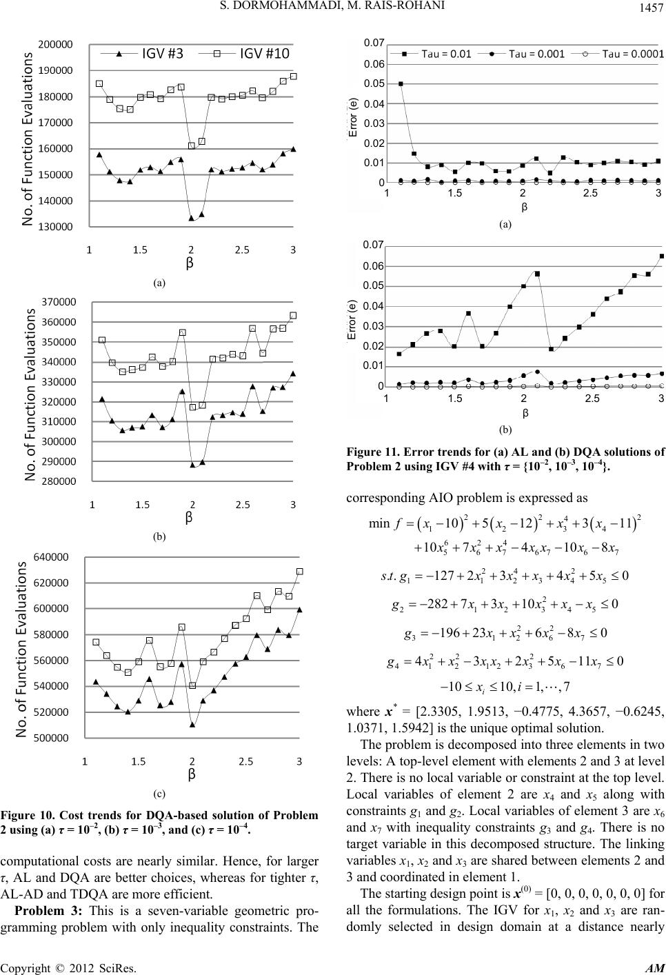

S. DORMOHAMMADI, M. RAIS-ROHANI 1457
(a)
(b)
(c)
Figure 10. Cost trends for DQA-based solution of Problem
2 using (a)τ = 10–2, (b) τ = 10–3, and (c) τ = 10–4.
computational costs are nearly similar. Hence, for larger
τ, AL and DQA are better choices, whereas for tighter τ,
AL-AD and TDQA are more efficient.
Problem 3: This is a seven-variable geometric pro-
gramming problem with only inequality constraints. The
0.07
0.06
0.05
0.04
0.03
0.02
0.01
0
Error
(
e
)
1 1.5 2 2.5 3
β
(a)
0.07
0.06
0.05
0.04
0.03
0.02
0.01
0
Error
(
e
)
1 1.5 2 2.5
3
β
(b)
Figure 11. Error trends for (a) AL and (b) DQA solutions of
Problem 2 using IGV #4 with τ = {10–2, 10–3, 10–4}.
corresponding AIO problem is expressed as
 
22
4
1234
624
56767 67
min 10512311
107410 8
fxxxx
xxxxx xx
  
 

2
5
0
24 2
11234
.. 1272345st gxxxxx

  
2
21234
282 73100gxxxxx
5


22
3126
196 23680gxxx
7
x


22 2
41212367
432511gxxxxxxx0

 
1010,1, ,7
i
xi

 
where x* = [2.3305, 1.9513, −0.4775, 4.3657, −0.6245,
1.0371, 1.5942] is the unique optimal solution.
The problem is decomposed into three elements in two
levels: A top-level element with elements 2 and 3 at level
2. There is no local variable or constraint at the top level.
Local variables of element 2 are x4 and x5 along with
constraints g1 and g2. Local variables of element 3 are x6
and x7 with inequality constraints g3 and g4. There is no
target variable in this decomposed structure. The linking
variables x1, x2 and x3 are shared between elements 2 and
3 and coordinated in element 1.
The starting design point is x(0) = [0, 0, 0, 0, 0, 0, 0] for
all the formulations. The IGV for x1, x2 and x
3 are ran-
domly selected in design domain at a distance nearly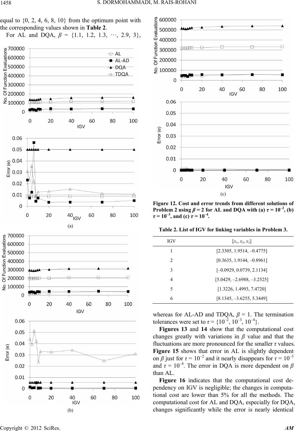

S. DORMOHAMMADI, M. RAIS-ROHANI
1458
equal to {0, 2, 4, 6, 8, 10} from the optimum point with
the corresponding values shown in Table 2.
For AL and DQA, β = {1.1, 1.2, 1.3, ···, 2.9, 3},
(a)
(b)
(c)
Figure 12. Cost and error trends from different solutions of
Problem 2 using β = 2 for AL and DQA with (a) τ = 10–2, (b)
τ = 10–3, and (c) τ = 10–4.
Table 2. List of IGV for linking variables in Problem 3.
IGV [x1, x2, x3]
1 [2.3305, 1.9514, –0.4775]
2 [0.3635, 1.9144, –0.8961]
3 [–0.0929, 0.0739, 2.1134]
4 [5.0429, –2.6988, –3.2525]
5 [1.3226, 1.4993, 7.4720]
6 [8.1345, –3.6255, 5.3449]
whereas for AL-AD and TDQA, β = 1. The termination
tolerances were set to τ = {10–2, 10–3, 10–4}.
Figures 13 and 14 show that the computational cost
changes greatly with variations in β value and that the
fluctuations are more pronounced for the smaller τ values.
Figure 15 shows that error in AL is slightly dependent
on β just for τ = 10–2 and it nearly disappears for τ = 10–3
and τ = 10–4. The error in DQA is more dependent on β
than AL.
Figure 16 indicates that the computational cost de-
pendency on IGV is negligible; the changes in computa-
tional cost are lower than 5% for all the methods. The
computational cost for AL and DQA, especially for DQA,
changes significantly while the error is nearly identical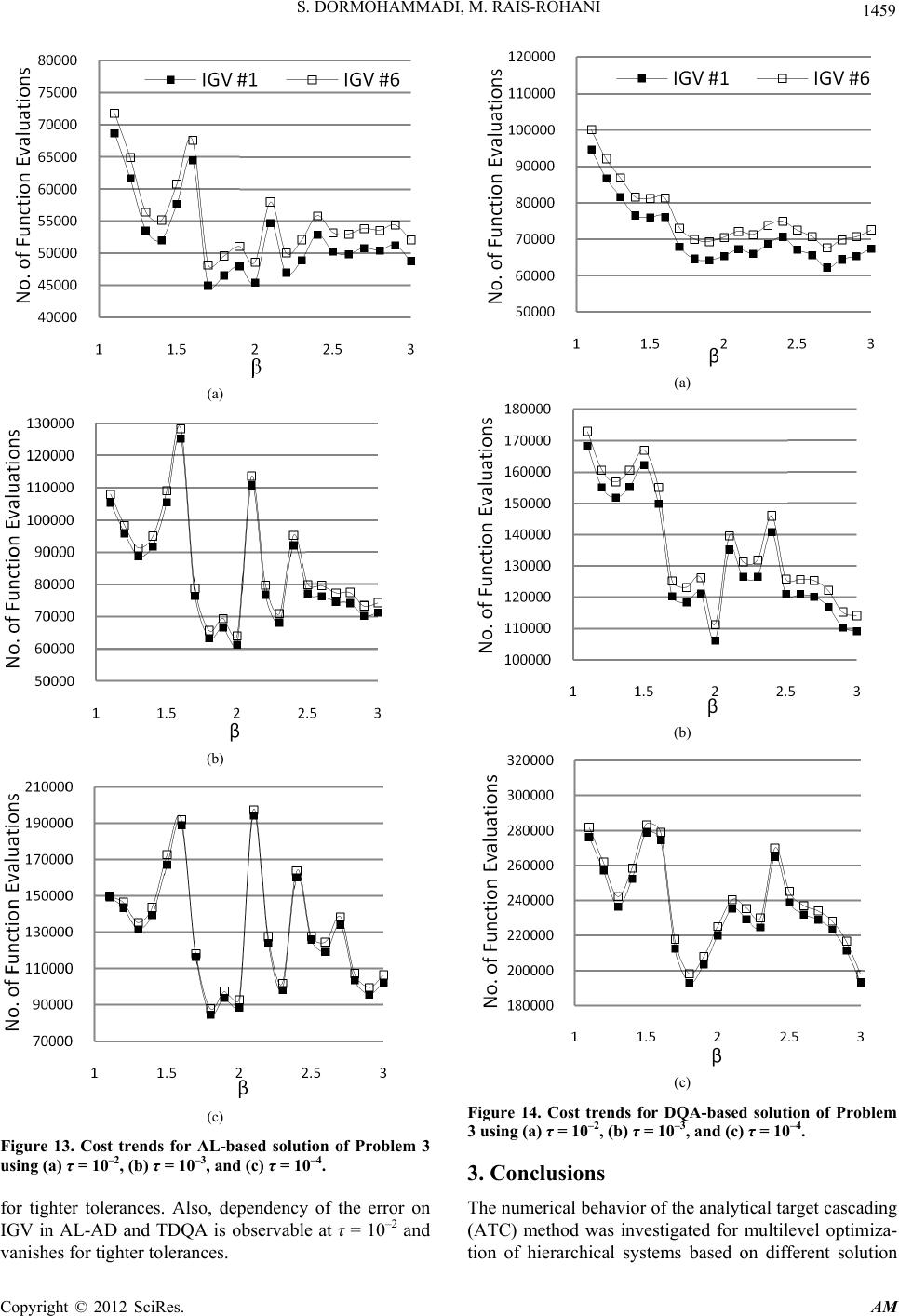

S. DORMOHAMMADI, M. RAIS-ROHANI 1459
(a)
(b)
(c)
Figure 13. Cost trends for AL-based solution of Problem 3
using (a) τ = 10–2, (b) τ = 10–3, and (c) τ = 10–4.
for tighter tolerances. Also, dependency of the error on
IGV in AL-AD and TDQA is observable at τ = 10–2 and
vanishes for tighter tolerances.
(a)
(b)
(c)
Figure 14. Cost trends for DQA-based solution of Problem
3 using (a) τ = 10–2, (b) τ = 10–3, and (c) τ = 10–4.
3. Conclusions
The numerical behavior of the analytical target cascading
(ATC) method was investigated for multilevel optimiza-
tion of hierarchical systems based on different solution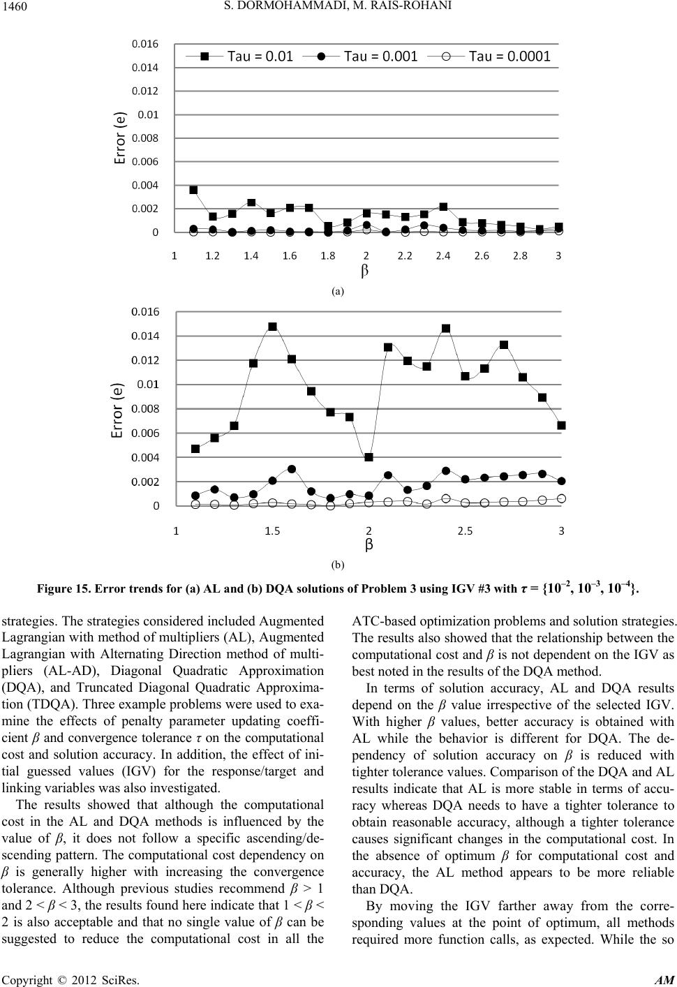

S. DORMOHAMMADI, M. RAIS-ROHANI
1460
(a)
(b)
Figure 15. Error trends for (a) AL and (b) DQA solutions of Problem 3 using IGV #3 with τ = {10–2, 10–3, 10–4}.
strategies. The strategies considered included Augmented
Lagrangian with method of multipliers (AL), Augmented
Lagrangian with Alternating Direction method of multi-
pliers (AL-AD), Diagonal Quadratic Approximation
(DQA), and Truncated Diagonal Quadratic Approxima-
tion (TDQA). Three example problems were used to exa-
mine the effects of penalty parameter updating coeffi-
cient β and convergence tolerance τ on the computational
cost and solution accuracy. In addition, the effect of ini-
tial guessed values (IGV) for the response/target and
linking variables was also investigated.
The results showed that although the computational
cost in the AL and DQA methods is influenced by the
value of β, it does not follow a specific ascending/de-
scending pattern. The computational cost dependency on
β is generally higher with increasing the convergence
tolerance. Although previous studies recommend β > 1
and 2 < β < 3, the results found here indicate that 1 < β <
2 is also acceptable and that no single value of β can be
suggested to reduce the computational cost in all the
ATC-based optimization problems and solution strategies.
The results also showed that the relationship between the
computational cost and β is not dependent on the IGV as
best noted in the results of the DQA method.
In terms of solution accuracy, AL and DQA results
depend on the β value irrespective of the selected IGV.
With higher β values, better accuracy is obtained with
AL while the behavior is different for DQA. The de-
pendency of solution accuracy on β is reduced with
tighter tolerance values. Comparison of the DQA and AL
results indicate that AL is more stable in terms of accu-
racy whereas DQA needs to have a tighter tolerance to
obtain reasonable accuracy, although a tighter tolerance
causes significant changes in the computational cost. In
the absence of optimum β for computational cost and
accuracy, the AL method appears to be more reliable
than DQA.
By moving the IGV farther away from the corre-
sponding values at the point of optimum, all methods
required more function calls, as expected. While the so

S. DORMOHAMMADI, M. RAIS-ROHANI 1461
(a)
(b)
(c)
Figure 16. Cost and error trends from different solutions of
Problem 3 using β = 2 for AL and DQA with (a) τ = 10–2, (b)
τ = 10–3, and (c) τ = 10–4.
lution accuracy in AL and DQA was not influenced by
the choice of IGV, the trend was quite the opposite for
AL-AD and TDQA as they both had great dependency
on IGV. The inner loop convergence requirement is more
costly for AL and DQA than TDQA and AL-AD. Fur-
thermore, the increase in computational cost for AL-AD
and TDQA is much greater than AL and DQA when IGV
is farther away from the optimum, but TDQA and AL-
AD still show better performance. AL-AD and TDQA
need tighter termination tolerances to have better accu-
racy.
In summary, the τ and β values have greater effect on
AL and DQA solutions than the other two coordination
strategies and they are not influenced by IGV. Hence, in
using AL and DQA, appropriate values for these two
parameters can enhance both solution accuracy and
computational cost. In contrast, the computational cost
and accuracy of AL-AD and TDQA are greatly depend-
ent on the IGV.
As part of the future work, the computational charac-
teristics of a newly developed approach based on the
exponential method of multipliers within the framework
of ATC will be investigated.

S. DORMOHAMMADI, M. RAIS-ROHANI
1462
4. Acknowledgements
The funding provided for this research by the National
Science Foundation under Grant No. CMMI-0826547 is
gratefully acknowledged.
REFERENCES
[1] N. F. Michelena, H. M. Kim and P. Y. Papalambros, “A
System Partitioning and Optimization Approach to Target
Cascading,” Proceedings of the 12th International Con-
ference on Engineering Design, Munich, 24-26 August
1999, pp. 1109-1112.
[2] H. M. Kim, N. F. Michelena, P. Y. Papalambros and T.
Jiang, “Target Cascading in Optimal System Design,” ASME
Transaction on Journal of Mechanical Design, Vol. 125,
2003, pp. 474-480. doi:10.1115/1.1582501
[3] H. M. Kim, N. F. Michelena, P. Y. Papalambros and T.
Jiang, “Target Cascading in Optimal System Design,” Pro-
ceedings of the 26th Design Automation Conference, Bal-
timore, 10-13 September 2000, pp. 293-302.
[4] H. M. Kim, M. Kokkolaras, L. S. Louca, G. J. Delagram-
matikas, N. F. Michelena, Z. S. Filipi, P. Y. Papalambros,
J. L. Stein and D. N. Assanis, “Target Cascading in Auto-
motive Vehicle Design: A Class 6 Truck Study,” Inter-
national Journal of Vehicle Design, Vol. 29, No. 3, 2002,
pp. 199-225. doi:10.1504/IJVD.2002.002010
[5] H. M. Kim, D. G. Rideout, P. Y. Papalambros and J. L.
Stein, “Analytical Target Cascading in Automotive Ve-
hicle Design,” Proceedings of ASME Design Engineering
Technical Conference and Computers and Information in
Engineering Conference, Pittsburgh, 9-12 September 2001,
pp. 661-670.
[6] N. F. Michelena, H. Park and P. Y. Papalambros, “Con-
vergence Properties of Analytical Target Cascading,” AIAA
Journal, Vol. 41, No. 5, 2003, pp. 897-905.
doi:10.2514/2.2025
[7] N. Tzevelekos, M. Kokkolaras, P. Y. Papalambros, M. F.
Hulshof, L. F. P. Etman and J. E. Rooda, “An Empirical
Local Convergence Study of Alternative Coordination
Schemes in Analytical Target Cascading,” Proceedings of
the 5th World Congress on Structural and Multidiscipli-
nary Optimization, Venice, 19-23 May 2003, pp. 1-6.
[8] J. J. Michalek and P. Y. Papalambros, “An Efficient
Weighting Update Method to Achieve Acceptable Incon-
sistency Deviation in Analytical Target Cascading,” Jour-
nal of Mechanical Design, Vol. 127, No. 2, 2005, pp. 206-
214. doi:10.1115/1.1830046
[9] J. J. Michalek and P. Y. Papalambros, “Weights, Norms,
and Notation in Analytical Target Cascading,” Journal of
Mechanical Design, Vol. 127, 2005, pp. 499-501.
doi:10.1115/1.1862674
[10] S. Tosserams, “Analytical Target Cascading: Convergence
Improvement by Subproblem Post-Optimality Sensitivi-
ties,” MS Thesis, Eindhoven University of Technology,
Eindhoven, 2004.
[11] D. P. Bertsekas, “Nonlinear Programming,” 2nd Edition,
Athena Scientific, Belmont, 2003.
[12] J. B. Lassiter, M. M. Wiecek and K. R. Andrighetti, “La-
grangian Coordination and Analytical Target Cascading:
Solving ATC-Decomposed Problems with Lagrangian-
Duality,” Optimization and Engineering, Vol. 6, No. 3,
2005, pp. 361-381.
doi:10.1007/s11081-005-1744-4
[13] V. Y. Blouin, J. Lassiter, M. Wiecek and G. M. Fadel,
“Augmented LagrangianCoordination for Decomposed
Design Problems,” 6th World Congresses of Structural and
Multidisciplinary Optimization, Rio de Janeiro, 30 May-3
June, 2005, pp. 1-10.
[14] H. M. Kim, W. Chen and M. M. Wiecek, “Lagrangian
Coordination for Enhancing the Convergence of Ana-
lytical Target Cascading,” AIAA Journal, Vol. 44, No. 10,
2006, pp. 2197-2207. doi:10.2514/1.15326
[15] S. Tosserams, L. F. P. Etman, P. Y. Papalambros and J. E.
Rooda, “An Augmented Lagrangian Relaxation for Ana-
lytical Target Cascading Using the Alternating Directions
Method of Multipliers,” Structural and Multidisciplinary
Optimization, Vol. 31, No. 3, 2006, pp. 176-189.
doi:10.1007/s00158-005-0579-0
[16] Y. Li, Z. Lu and J. J. Michalek, “Diagonal Quadratic
Approximation for Parallelization of Analytical Target
Cascading,” Journal of Mechanical Design, Vol. 130, 2008,
pp. 051402-1-051402-11.
[17] W. Wang, V. Y. Blouin, M. Gardenghi, M. M. Wiecek, G.
M. Fadel and B. Sloop, “A Cutting Plane Method For
Analytical Target Cascading With Augmented Lagran-
gian Coordination,” Proceedings of the ASME Interna-
tional Design Engineering Technical Conferences &
Computers and Information in Engineering Conference
IDETC/CIE, Montreal, 15-18 August 2010, pp. 791-800.