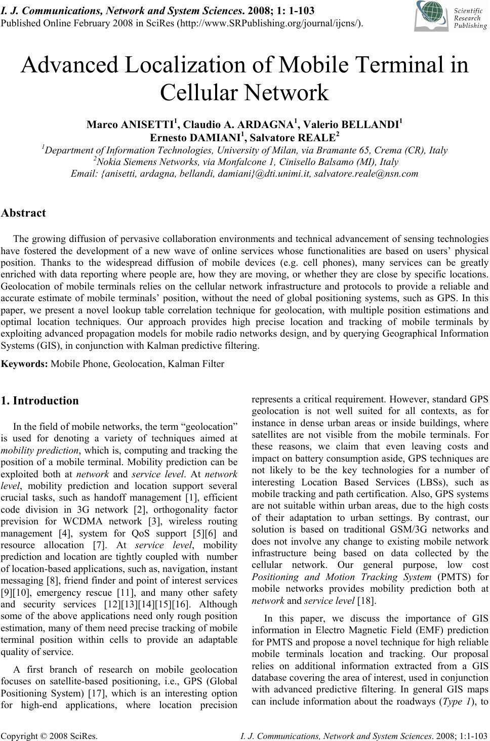I. J. Communications, Network and System Sciences. 2008; 1: 1-103
Published Online February 2008 in SciRes (http://www.SRPublishing.org/journal/ijcns/).
Copyright © 2008 SciRes. I. J. Communications, Network and System Sciences. 2008; 1:1-103
Advanced Localization of Mobile Terminal in
Cellular Network
Marco ANISETTI1, Claudio A. ARDAGNA1, Valerio BELLANDI1
Ernesto DAMIANI1, Salvatore REALE2
1Department of Information Technologies, University of Milan, via Bramante 65, Crema (CR), Italy
2Nokia Siemens Networks, via Monfalcone 1, Cinisello Balsamo (MI), Italy
Abstract
The growing diffusion of pervasive collaboration environments and technical advancement of sensing technologies
have fostered the development of a new wave of online services whose functionalities are based on users’ physical
position. Thanks to the widespread diffusion of mobile devices (e.g. cell phones), many services can be greatly
enriched with data reporting where people are, how they are moving, or whether they are close by specific locations.
Geolocation of mobile terminals relies on the cellular network infrastructure and protocols to provide a reliable and
accurate estimate of mobile terminals’ position, without the need of global positioning systems, such as GPS. In this
paper, we present a novel lookup table correlation technique for geolocation, with multiple position estimations and
optimal location techniques. Our approach provides high precise location and tracking of mobile terminals by
exploiting advanced propagation models for mobile radio networks design, and by querying Geographical Information
Systems (GIS), in conjunction with Kalman predictive filtering.
Keywords: Mobile Phone, Geolocation, Kalman Filter
1. Introduction
In the field of mobile networks, the term “geolocation”
is used for denoting a variety of techniques aimed at
mobility prediction, which is, computing and tracking the
position of a mobile terminal. Mobility prediction can be
exploited both at network and service level. At network
level, mobility prediction and location support several
crucial tasks, such as handoff management [1], efficient
code division in 3G network [2], orthogonality factor
prevision for WCDMA network [3], wireless routing
management [4], system for QoS support [5][6] and
resource allocation [7]. At service level, mobility
prediction and location are tightly coupled with number
of location-based applications, such as, navigation, instant
messaging [8], friend finder and point of interest services
[9][10], emergency rescue [11], and many other safety
and security services [12][13][14][15][16]. Although
some of the above applications need only rough position
estimation, many of them need precise tracking of mobile
terminal position within cells to provide an adaptable
quality of service.
A first branch of research on mobile geolocation
focuses on satellite-based positioning, i.e., GPS (Global
Positioning System) [17], which is an interesting option
for high-end applications, where location precision
represents a critical requirement. However, standard GPS
geolocation is not well suited for all contexts, as for
instance in dense urban areas or inside buildings, where
satellites are not visible from the mobile terminals. For
these reasons, we claim that even leaving costs and
impact on battery consumption aside, GPS techniques are
not likely to be the key technologies for a number of
interesting Location Based Services (LBSs), such as
mobile tracking and path certification. Also, GPS systems
are not suitable within urban areas, due to the high costs
of their adaptation to urban settings. By contrast, our
solution is based on traditional GSM/3G networks and
does not involve any change to existing mobile network
infrastructure being based on data collected by the
cellular network. Our general purpose, low cost
Positioning and Motion Tracking System (PMTS) for
mobile networks provides mobility prediction both at
network and service level [18].
In this paper, we discuss the importance of GIS
information in Electro Magnetic Field (EMF) prediction
for PMTS and propose a novel technique for high reliable
mobile terminals location and tracking. Our proposal
relies on additional information extracted from a GIS
database covering the area of interest, used in conjunction
with advanced predictive filtering. In general GIS maps
can include information about the roadways (Type 1), to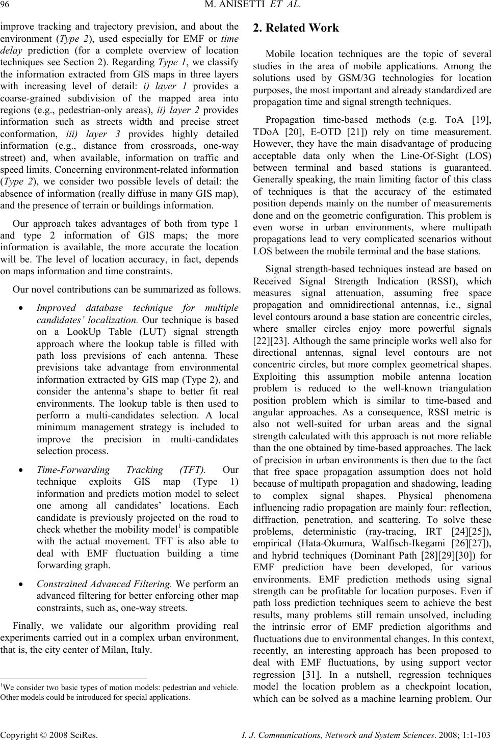

96 M. ANISETTI ET AL.
Copyright © 2008 SciRes. I. J. Communications, Network and System Sciences. 2008; 1:1-103
improve tracking and trajectory prevision, and about the
environment (Type 2), used especially for EMF or time
delay prediction (for a complete overview of location
techniques see Section 2). Regarding Type 1, we classify
the information extracted from GIS maps in three layers
with increasing level of detail: i) layer 1 provides a
coarse-grained subdivision of the mapped area into
regions (e.g., pedestrian-only areas), ii) layer 2 provides
information such as streets width and precise street
conformation, iii) layer 3 provides highly detailed
information (e.g., distance from crossroads, one-way
street) and, when available, information on traffic and
speed limits. Concerning environment-related information
(Type 2), we consider two possible levels of detail: the
absence of information (really diffuse in many GIS map),
and the presence of terrain or buildings information.
Our approach takes advantages of both from type 1
and type 2 information of GIS maps; the more
information is available, the more accurate the location
will be. The level of location accuracy, in fact, depends
on maps information and time constraints.
Our novel contributions can be summarized as follows.
• Improved database technique for multiple
candidates’ localization. Our technique is based
on a LookUp Table (LUT) signal strength
approach where the lookup table is filled with
path loss previsions of each antenna. These
previsions take advantage from environmental
information extracted by GIS map (Type 2), and
consider the antenna’s shape to better fit real
environments. The lookup table is then used to
perform a multi-candidates selection. A local
minimum management strategy is included to
improve the precision in multi-candidates
selection process.
• Time-Forwarding Tracking (TFT). Our
technique exploits GIS map (Type 1)
information and predicts motion model to select
one among all candidates’ locations. Each
candidate is previously projected on the road to
check whether the mobility model1 is compatible
with the actual movement. TFT is also able to
deal with EMF fluctuation building a time
forwarding graph.
• Constrained Advanced Filtering. We perform an
advanced filtering for better enforcing other map
constraints, such as, one-way streets.
Finally, we validate our algorithm providing real
experiments carried out in a complex urban environment,
that is, the city center of Milan, Italy.
1We consider two basic types of motion models: pedestrian and vehicle.
Other models could be introduced for special applications.
2. Related Work
Mobile location techniques are the topic of several
studies in the area of mobile applications. Among the
solutions used by GSM/3G technologies for location
purposes, the most important and already standardized are
propagation time and signal strength techniques.
Propagation time-based methods (e.g. ToA [19],
TDoA [20], E-OTD [21]) rely on time measurement.
However, they have the main disadvantage of producing
acceptable data only when the Line-Of-Sight (LOS)
between terminal and based stations is guaranteed.
Generally speaking, the main limiting factor of this class
of techniques is that the accuracy of the estimated
position depends mainly on the number of measurements
done and on the geometric configuration. This problem is
even worse in urban environments, where multipath
propagations lead to very complicated scenarios without
LOS between the mobile terminal and the base stations.
Signal strength-based techniques instead are based on
Received Signal Strength Indication (RSSI), which
measures signal attenuation, assuming free space
propagation and omnidirectional antennas, i.e., signal
level contours around a base station are concentric circles,
where smaller circles enjoy more powerful signals
[22][23]. Although the same principle works well also for
directional antennas, signal level contours are not
concentric circles, but more complex geometrical shapes.
Exploiting this assumption mobile antenna location
problem is reduced to the well-known triangulation
position problem which is similar to time-based and
angular approaches. As a consequence, RSSI metric is
also not well-suited for urban areas and the signal
strength calculated with this approach is not more reliable
than the one obtained by time-based approaches. The lack
of precision in urban environments is then due to the fact
that free space propagation assumption does not hold
because of multipath propagation and shadowing, leading
to complex signal shapes. Physical phenomena
influencing radio propagation are mainly four: reflection,
diffraction, penetration, and scattering. To solve these
problems, deterministic (ray-tracing, IRT [24][25]),
empirical (Hata-Okumura, Walfisch-Ikegami [26][27]),
and hybrid techniques (Dominant Path [28][29][30]) for
EMF prediction have been developed, for various
environments. EMF prediction methods using signal
strength can be profitable for location purposes. Even if
path loss prediction techniques seem to achieve the best
results, many problems still remain unsolved, including
the intrinsic error of EMF prediction algorithms and
fluctuations due to environmental changes. In this context,
recently, an interesting approach has been proposed to
deal with EMF fluctuations, by using support vector
regression [31]. In a nutshell, regression techniques
model the location problem as a checkpoint location,
which can be solved as a machine learning problem. Our

ADVANCED LOCALIZATION OF MOBILE TERMINAL IN CELLULAR NETWORK 97
Copyright © 2008 SciRes. I. J. Communications, Network and System Sciences. 2008; 1:1-103
approach, however, does not rely on a training phase,
since real data sampling are not available everywhere.
Furthermore, we focus on tracking and on dense
localization, where checkpoint and neural network based
strategies are not suitable. Specially, we rely on the basic
techiniques outlined below.
Database correlation. This technique relies on a
database built on RSSI predictions or measurements.
Mobile terminals positions are determined by evaluating
RSSI measurements, which are performed by individual
terminals or even by the BSs. The measurements are
compared with the entries in the database. The
corresponding correlation calculations find out the
database entry that better matches the measurements lead
to a location estimation [32][33]. Our approach basically
relies on the principle of database correlation. Much in
line with the RADAR system developed by Microsoft
research [34] for wireless networks, our method uses a
LUT for multiple candidates’ selection. Differently from
RADAR, however, we select the number of candidates
depending on the sensibility of the region and on GIS
information.
Filtering. Using triangulation and database correlation,
the intrinsic location error of RSSI is never taken into
account. Many recent works are aimed at overcoming this
problem using Kalman filtering techniques with mobile
motion model and RSSI triangulation. One interesting
work [39] treats the problem of mobility in ATM network.
It develops a hierarchical user mobility model that closely
represents the movement behavior of a mobile user, and
uses pattern matching and Kalman filtering, yielding to an
accurate location prediction algorithm. Another work [40]
proposes two algorithms for real-time tracking, location,
and dynamic motion of a mobile station in a cellular
network. This method is based on pre-filtering and two
Kalman filters (one to estimate the discrete command
process and the other to estimate the mobility state). The
mobility model is built on a dynamic linear system driven
by a discrete command process that was originally
developed for tracking maneuvering targets in tactical
weapons system [35][36]. The command process is
modeled as a semi-Markov process over a finite set of
acceleration levels, as in [37]. The filtering technique,
presented in our work does not filter the location of
mobile using RSSI [37][38], but it takes the most
probable position filtered by our Time Forwarding
Tracking (TFT) technique and tries to enforce the map
and motion model constraints. Therefore, our filtering
technique is well distinct from the ones introduced above,
even if it exploits a similar motion model.
3. EMF Prediction with Antennas’ Shape
EMF prediction is a crucial task for those location
strategies relying on triangulation or lookup table over
RSSI. The amount of GIS information available (Type 2
from GIS map) drives the choice among a number of
applicable algorithms. In this paper, we adopt Hata-
Okumura [26] for prediction in absence of environmental
information and COST231 Wallfisch-Ikegami [27] to
take into account the shapes of the buildings. The statistic
prediction model COST231 is only suitable for simulated
environment where antennas are supposed to be omni-
directional. In our previous works, we adopted this
approach for EMF prediction, obtaining very good results
in a simulated urban environment [39][40]. In real
environment, however, this omni-directionality cannot be
assumed without a loss in EMF estimation quality, since
real antennas’ shape have a big impact on EMF prediction.
There are two ways to deal with real antennas’ shapes: i)
use a deterministic ray-tracing, ii) introduce shapes in
statistical EMF prediction. Here, we propose a variation
of COST231 that includes a simple notion of antenna
shape to better estimate the EMF. The deterministic ray
tracing techniques in fact suffer of several problems, as
for instance burdensome time-complexity need for a high
precision antenna database, which make them not suitable
for our approach. We model the shape of the antenna as a
simple function Sa of the direction angle, Sa:[0…360] →
[0…Maxloss], where Maxloss is the maximum loss
defined for a certain type of antenna. Function Sa(α) maps
degree α to the loss due to the shape of the antenna a;
such loss depends upon the angle of the point where the
field is measured with respect to the antenna’s main axes.
As an example, using our shape function inside
COST231, the path loss of point p over the map, with
respect to antenna a, is defined as follow:
badd llPATHLOSS += (1)
where ladd=Sa(α) represents the additional loss produced
by the shape of the antenna a, with α the angle identified
by point p and the principal direction of antenna a, and lb
is the component of canonical COST231 (i.e., either LOS
or NLOS). Fig. 1 shows a comparison between EMF
predicted with buildings structure and omni-directional
antennas and EMF predicted with buildings structure and
directional antennas.
Figure 1. Comparison between omni-directional antennas
and directional antennas.
The availability of information about the shapes and
directions of the antennas, as well as more information on
the environment, allows of significantly improving the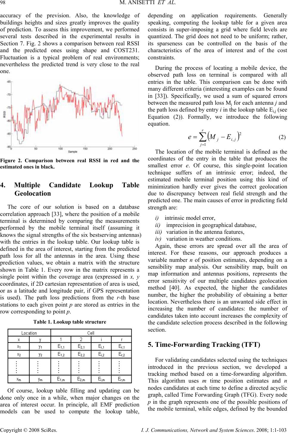

98 M. ANISETTI ET AL.
Copyright © 2008 SciRes. I. J. Communications, Network and System Sciences. 2008; 1:1-103
accuracy of the prevision. Also, the knowledge of
buildings heights and sizes greatly improves the quality
of prediction. To assess this improvement, we performed
several tests described in the experimental results in
Section 7. Fig. 2 shows a comparison between real RSSI
and the predicted ones using shape and COST231.
Fluctuation is a typical problem of real environments;
nevertheless the predicted trend is very close to the real
one.
Figure 2. Comparison between real RSSI in red and the
estimated ones in black.
4. Multiple Candidate Lookup Table
Geolocation
The core of our solution is based on a database
correlation approach [33], where the position of a mobile
terminal is determined by comparing the measurements
performed by the mobile terminal itself (assuming it
knows the signal strengths of the six bestserving antennas)
with the entries in the lookup table. Our lookup table is
defined in the area of interest, starting from the predicted
path loss for all the antennas in the area. Using these
prediction values, we obtain a matrix with the structure
shown in Table 1. Every row in the matrix represents a
single point within the coverage area (expressed in x, y
coordinates, if 2D cartesian representation of area is used,
or as a latitude and longitude pair, if GPS representation
is used). The path loss predictions from the r-th base
stations to each given point p are stored as entries in the
row corresponding to point p.
Table 1. Lookup table structure
Of course, lookup table filling and updating can be
done only once in a while, when major changes on the
area of interest occur. In principle, all EMF prediction
models can be used to compute the lookup table,
depending on application requirements. Generally
speaking, computing the lookup table for a given area
consists in super-imposing a grid where field levels are
quantized. The grid does not need to be uniform; rather,
its sparseness can be controlled on the basis of the
characteristics of the area of interest and of the cost
constraints.
During the process of locating a mobile device, the
observed path loss on terminal is compared with all
entries in the table. This comparison can be done with
many different criteria (interesting examples can be found
in [33]). Specifically, we used a sum of squared errors
between the measured path loss Mj for each antenna j and
the path loss defined by entry i in the lookup table Ei,j (see
Equation (2)). Formally, we introduce the following
equation.
()
∑
=
−= r
j
jij EMe
1
2
, (2)
The location of the mobile terminal is defined as the
coordinates of the entry in the table that produces the
smallest error e. Of course, this single-point location
technique suffers of an intrinsic error; indeed, the
estimated mobile terminal position using this kind of
minimization hardly ever gives the correct geolocation
due to discrepancy between real field strength and the
predicted one. The main causes of error in predicting field
strength are:
i) intrinsic model error,
ii) imprecision in geographical database,
iii) variation in the antenna features,
iv) variation in weather conditions.
Again, these errors are spread over all the area of
interest. For these reasons, our approach produces a
variable number n of position estimates, depending on a
sensibility map analysis. Our sensibility map, built on
map information and antennas positions, represents the
error sensitivity of our multiple candidates geolocation
method [40]. As expected, the higher the candidates
number, the higher the probability of obtaining a better
location. Nevertheless there is an unwanted side effect in
increasing the number of candidates: the number of
candidates taken into account increases the complexity of
the candidate selection process described in the following
section.
5. Time-Forwarding Tracking (TFT)
For validating candidates selected using the techniques
introduced in the previous section, we developed a
tracking method based on a time-forwarding algorithm.
This algorithm uses m time position estimates and n
nodes candidates at each time to define a directed acyclic
graph, called Time Forwarding Graph (TFG). Every node
p in the graph represents one of the possible positions of
the mobile terminal, while edges, defined by the bounded

ADVANCED LOCALIZATION OF MOBILE TERMINAL IN CELLULAR NETWORK 99
Copyright © 2008 SciRes. I. J. Communications, Network and System Sciences. 2008; 1:1-103
nodes (source and destination nodes), represent motion
between them. Each edge has associated a weight that is
computed based on reachability and map constraints. In
our previous work [40], this weight was defined by taking
into account the estimated velocity and acceleration at the
source node, and by evaluating the reachable velocity and
acceleration considering the position of the destination
node. The obtained values were then compared with
information inferred from the map. Of course, this type of
advanced function works well when a reasonable upper
bound to the position error can be assumed. Since in this
paper we deal with real (as opposed to lab) environments,
an acceptable error for every position cannot be
guaranteed. Therefore the aforesaid weighting techniques
cannot be applied. We then adopt a simpler weighting
technique postponing the refinement to the filtering stage.
At this stage, we only evaluate the edge weight to exclude
the unreachable nodes. Therefore the weight function W
is defined over an edge e = (pi,t, pj,t+k) as follows:
⎩
⎨
⎧
∞+
≤
=otherwise
kThmapeifmape
mapeW )( ),( ),( ),(
µµ
(3)
where i,j
∈ [1,…,n] and k ∈ [1,…,m]. The function µ
calculates the real distance between two nodes pi,t and
pj,t+k taking into account the map (presence of buildings,
street curves and so on). The threshold Th(k) defines the
maximum acceptable distance between each node and it is
a function of the time variation k. Using this approach the
weights of the edges are in linear relation with the nodes
distances. Considering the real environment fluctuation
and the fact that the sampling interval is very short (≈500
ms), this assumption is realistic enough for TFT filtering
purpose2. Summarizing each edge of the graph has a
weight that defines the reachability between the bounded
nodes. All maps and motion constraints are enforced by
the weight function. By searching the minimum path on
the graph (i.e., the path from time t to time t+m with
minimum weight), we obtain a preliminary filtered
position for the mobile (the nodes included in the
obtained path). In our previous work, we used a different
weight function that worked using k = 1, meaning that
there were no edge between non-temporal consecutive
nodes.
Once again, we remark that, in real applications, the
assumption of a bounded error is too restrictive, and a set
of candidates’ nodes can be completely unreachable due
to the fluctuation effect. Therefore our TFG needs to take
into account also this noise effect. Every node p of the
TFG is then associated with a set of nodes St at certain
time t as follows:
[]
tntttpppS ,,2,1 ,,, L= (4)
2 To the best of our knowledge the probability of having an overlapped
estimation, over time, is high only in the case of stationary mobile
device.
St represents the set of the n candidates positions for time
t. The distance from a node pi,t to a node pj,t+k is the same
as the weight W among them. The distance can be also
defined from a node pi,t and a set of nodes St+k as follow:
[]
)),,((min),,( ,,1, mapppmapSpM ktjtinjktti +∈+ = µ
L
(5)
where M is a distance function from node pi,t to set St+k
according to the map. In our TFG graph, two types of
edges exist:
• edges e between two consecutive nodes, if
W≠+∞.
• forwarding edges e between two non temporal
consecutive nodes. pi,t and pj,t+k, if
M(pi,t,St+k,map)≠+∞ and
minh=1..k-1(M(pi,t,St+h,map) =+∞.
Fig. 3 shows the TGF. Note that in our approach, the
choice of parameter m becomes critical. On the one hand,
using a high m (i.e., long time prevision), we obtain a
“strong trend” prevision that filters out any out-of-trend
movement. This result is not acceptable in pedestrian-
only areas like a city square, where motion can well be
chaotic without any prevalent movement trend. On the
other hand, a value too small for m could cause an error
dependency, which in turn could produce bad results in
high trend-correlation areas like motorways or one-way
streets. However, since layer 1 map information permits
to distinguish between pedestrian-only areas and
motorways, it becomes adequately possible to tune
parameter m.3 In this way, we obtain a map correlation of
our first-level movement estimates, and we can
substantially improve the tracking quality of our lookup
table technique (see Section 7 for details).
Figure 3. Graph through example for time-forwards
tracking. In red the selected position nodes and the selected
path, in black the possible position nodes. The dotted line
shows an example of an edge between two non consecutive
nodes.
3 A similar dynamic tuning of parameter m can be based on the
characteristics of user’s vehicle.

100 M. ANISETTI ET AL.
Copyright © 2008 SciRes. I. J. Communications, Network and System Sciences. 2008; 1:1-103
Our time-forwarding tracking technique takes full
advantage from all available GIS information, such as
area classification, so that validation of candidates’
locations depends on map constraints. In many cases, the
additional information provided by the map is poor or
absent; when this happens, our technique is able to
dynamically build an information database by estimating
all relevant knowledge including speed and acceleration.
6. Tracking with Constrained Kalman
Filtering
Using the time-forwarding tracking technique
explained in the previous section, we obtain a trusted
location measurement zk at time k, which complies with
all map constraints taken into account by TFT. This
location zk can be associated with a state Xk=[x,y,x',y']T of
our mobile device at certain time k, where x and y are the
position coordinates and x' and y' define the velocity
vector. In general, this state defines a movement trend
that already has high confidence and low error, if
compared with the actual mobile antenna path (see Fig. 5).
To increase its quality, this movement trend is filtered
with constrained Kalman filter (CKF) [41], obtaining a
robust error and time-deep prevision tracking (Fig. 4
shows our CKF architecture).
The Kalman filter module (the white box in Fig. 4) has
the following input: i) state position measure zk from TFT
that use map layer 1, ii) the uk-1 control input provided by
HSMM (Hidden Semi-Markov Model) module, used also
in [40], and defined using also map layer 3, iii)
constrained function defined on map layer 2. One of the
main advantages of this filtering is that it takes into
account both measurement error and system error; besides,
this one previous-state dependency filtering becomes very
usable in real time tracking environment. The Kalman
state equation shown in Fig. 4 is defined using the
following fundamental matrixes:
⎥
⎥
⎥
⎥
⎦
⎤
⎢
⎢
⎢
⎢
⎣
⎡
=
1000
0100
010
001
T
T
A (6)
⎥
⎥
⎥
⎥
⎥
⎥
⎦
⎤
⎢
⎢
⎢
⎢
⎢
⎢
⎣
⎡
=
T
T
T
T
B
0
0
2
0
0
22
2
(7)
⎥
⎦
⎤
⎢
⎣
⎡
=0010
0001
C (8)
where T is the time interval between two consecutive
observations.
The work [40] proposes to use simple Kalman filtering
with HSMM module for location in wireless network.
The main difference between this approach and ours is
that we filter only motion errors and inertia oversight, but
we do not filter the error introduced by signal strength
prevision. Indeed, the position estimate used to correct
the Kalman prevision is already compatible with map
constraints and motion characteristics of the mobile
antenna. Using this filtering, we improve the accuracy of
the mobile terminal’s location.
Figure 4. Constrain Kalman filtering architecture.
7. Experimental Results
Using three different cellular phones and a GPS
antenna, we performed five trips in downtown Milan,
over a month of experimentation. The city area we chose,
which is near the railway station called Milano Centrale,
includes a non-uniform urban environment, with a park
and some skyscrapers. All trips were performed both by
car and on foot, and had duration varied from 5 minutes
to 1 hour. During these trips, information related to
serving and neighboring cells coupled with GPS latitude
and longitude were collected every 480 ms. We
performed two different types of testing, one for
evaluating EMF prediction quality and another for
assessing geolocation quality with respect to the actual
position of a moving cellular phone. Specially, we
emphasize the relation between the amount of available
environmental information and the quality of predicted
EMF. Environmental information is costly to collect and
is not likely to be available everywhere.
Since our aim is to locate mobile phones, we also
investigated the relation between EMF prediction and the
amount of filtering. More specifically, in the first type of
experiments, we computed EMF using different
combinations of information taken from our Type 2 GIS

ADVANCED LOCALIZATION OF MOBILE TERMINAL IN CELLULAR NETWORK 101
Copyright © 2008 SciRes. I. J. Communications, Network and System Sciences. 2008; 1:1-103
map. Selected combinations are: i) antenna’s shape with
no environmental information (LOS), ii) some
environmental information (buildings structure, with
fixed elevation) but no antenna shape (NLOS), iii)
environmental information and antenna’s shape
(NLOS+S), and iv) all information, including buildings
elevation and shape (NLOS+S+E).
Figure 5. A comparison between some of lookup table
candidate(square symbol), geolocation after filtering (cross
symbol) and real position presented in blac k dot.
The results presented in Table 2 show that the quality
in EMF prediction depends on the amount of type 2 GIS
information available. When all information is available,
the mean and variance of the error in EMF prediction is
highly reduced.
Table 2. Comparison of Mean Error in EMF Prediction. For
sake Of Conciseness, Mean and Variance (in Db) are
presented considering a subset of our experimens also
number of involved antennas (Ant.) and duration of the trip
(Dur) are presented.
In the second type of experiments, we present our
results in terms of location quality, showing their relation
with the available information and thus with the predicted
EMF. In our previous work [43], we investigated the
quality of our location approach in a simulated
environment achieving encouraging results. Here, we
evaluate the relation between quality of location and
amount of information available. Table 3 shows our
results; it is clear that our filtering strategy, which relies
on map information, can be fruitfully applied only when
all environmental information is available.
Table 3. Comparison of Mean Error Using our Location
algorithm
To conclude, the overall precision of our location
techniques is suitable for many location-based services
and applications even in a highly diverse urban
environment.
8. Conclusion
We have investigated the problem of mobile terminals
location in urban environments, analyzing some existing
location algorithms, and proposing a novel way to
improve location accuracy. Our approach employs a time-
forward tracking algorithm with GIS map constraints and
a constrained Kalman filtering for error correction
purposes. A complete experimentation confirms that
detailed GIS information can produce highly precise
location even using a simple statistical EMF prediction.
9. References
[1] H. Lin, R. Juang, and D. Lin, “Validation of an
improved locayionbased algorithm using gsm
measurement data,” IEEE Trans. Mobile Computing,
vol. 4, pp. 530 – 536, September - October 2005.
[2] H. Buddendick, G. WÖlfle, S. Burger, and P. Wertz,
“Simulator for performance analysis in umts fdd
networks with hsdpa,” 15th IEEE International
Symposium on Personal, Indoor and Mobile Radio
Communications (PIMRC), Barcelona, Spain,
September 2004.
[3] S. Burger, H. Buddendick, G. WÖlfle, and P. Wertz,
“Location dependent cdma orthogonality in system
level simulations,” 61st IEEE Vehicular Technology
Conference (VTC), Stockholm, Sweden, May 2005.
[4] L. Blazevic, J. L. Boudec, and S. Giordano, “A
location-based routing method for mobile ad hoc
networks,” IEEE Trans. Mobile computing, pp. 97–
110, March - April 2005.
[5] W. S. Soh and K. Kim, “QoS provisioning in
cellular networks based on mobility prediction
techiniques,” IEEE Comm.Magazine, vol. 41(1), pp.
86–112, January 2003.
[6] A. Aljadhai and T. Znati, “Predictive mobility
support for qos provisioning in mobile wireless
environments,” IEEE Journal Selected Areas in
Communications, pp. 1915 – 1930, October 2001.
[7] J. Chan and A. Seneviretne, “A pratical user
mobility prediction algorithm for supporting
adaptive qos in wireless networks,” Proc. IEEE
International Conference Networks (ICON’99), pp.
104 – 111, 1999.
[8] A. J .H. Peddemors, M. M. Lankhorst, J. de Heer,
“Presence, location, and instant messaging in a

102 M. ANISETTI ET AL.
Copyright © 2008 SciRes. I. J. Communications, Network and System Sciences. 2008; 1:1-103
context-aware application framework,” in Proc. of
the 4th International Conference on Mobile Data
Management (MDM), Melbourne, Australia,, 2003.
[9] CellSpotting.com, http://www.cellspotting.com.
[10] World-tracker.com, http://www.world-tracker.com/.
[11] (14 Jan 2004) Us fcc enhanced 911 fac sheet 2001.
[Online]. Available:
http://www.fcc.gov/911/enhanced/release/factsheet
requirements 012001.pdf
[12] MapAmobile, http://www.mapamobile.com/.
[13] N. Marmasse and C. Schmandt, “Safe & sound a
wireless leash,” in Proc. of CHI 2003, extended
abstract, 2003.
[14] N. Marmasse and C. Schmandt, “User-centered
location awareness,” IEEE Computer, vol. 37, no.
10, pp. 110–111, 2004.
[15] Teen Arrive Alive, http://www.teenarrivealive.com.
[16] C.A. Ardagna, M. Cremonini, E. Damiani, S. De
Capitani di Vimercati, and P. Samarati, “Supporting
location-based conditions in access control policies,”
in Proc. of the ACM Symposium on Information,
Computer and Communications Security
(ASIACCS’06), Taipei, Taiwan, March 2006.
[17] E. Kapplan, Understanding GPS: Principles and
Applications. Amsterdam, Netherlands: Elsevier,
1996.
[18] N. Samaan and A. Karmouch, “A mobility
prediction architecture based on contextual
knowledge and spatial conceptual maps,” IEEE
Trans. Mobile Computing, vol. 4, pp. 537 – 550,
November - December 2005.
[19] C. Drane, M. Macnaughtan, and C. Scott,
“Positioning gsm telephones,” IEEE Comm. Mag.,
vol. 46, pp. 46 – 55, Apr 1998
[20] J. J. Caffery and G. L. Stüber, “Overview of
radiolocation in cdma cellular systems,” IEEE
Communications Magazine, April 1998.
[21] M. Spirito, “On the accurancy of cellular mobile
station location estimation,” IEEE Trans. Veh.
Technol., vol. 50, pp. 3674 – 3685, May 2001
[22] W. Figel, N. shepherd, and W. Trammell, “Vehicle
location by a signal attenuation method,” IEEE Tans.
Veh. Technol., vol. VT - 18, pp. 105 – 110,
November 1969.
[23] H. song, “Automatic vehicle location in cellular
communications systems,” IEEE Tans. Veh.
Technol., vol. 43, pp. 902 – 908, November 1994.
[24] R. Hoppe, G. WÖlfle, and F. Landstorfer, “Fast 3-d
ray tracing for the planning of microcells by
intelligent preprocessing of the data base,” 3rd
European Personal and Mobile Communication
Conference (EPMCC), Paris, March 1999.
[25] G. WÖlfle, R. Hoppe, and F. Landstorfer, “A fast
and enhanced ray optical propagation model for
indoor and urban scenarios, based on an intelligent
preprocessing of the database,” 10th IEEE PIMRC,
Osaka, September 1999.
[26] Y. Okumura, E. Ohmori, T. Kawano, and K. Fukuda,
“Okumura-hata propagation prediction model for
uhf range, in the prediction methods for the
terrestrial land mobile service in the vhf and uhf
bands,” ITU-R Recommendation P.529-2, Geneva:
ITU, 1995.
[27] E. Damosso, “Cost 231: (digital mobile radio
towards future generation systems),” Final report,
European Comission, Bruxelles, 1999.
[28] G. WÖlfle, R. Wahl, P. Wertz, P. Wildbolz, and F.
Landstorfer, “Dominant path prediction model for
indoor scenarios,” German Microwave Conference
(GeMIC), April 2005.
[29] G. WÖlfle, R. Wahl, P. Wildbolz, and P. Wertz,
“Dominant path prediction model for indoor and
urban scenarios,” Duisburg (Germany), September
2004.
[30] R. Wahl, G. WÖlfle, P. Wertz, and P. Wildbolz,
“Dominant path prediction model for urban
scenarios,” 14th IST Mobile and Wireless
Communications Summit, Dresden (Germany), June
2005.
[31] Z. li Wu, C. hung Li, J. K.-Y. Ng, and K. R. Leung,
“Location estimation via support vector regression,”
IEEE Transactions on Mobile Computing,vol. 6,
March 2007.
[32] D. Zimmermmann, P. Wertz, J. Bauknecht, and
F.Landstorfer, “Performance of location methods in
an urban mobile communication network,”
Technical report, 2004.
[33] D. Zimmermmann, J. Baumann, M. Layh, F.
Landstorfer, R. Hoppe, and G. WÖlfle, “Database
correlection for positioning of mobile terminals in
cellular networks using wave propagation models,”
IEEE Vehicoular technology conference (VTC), Los
Angeles USA, October 2004.
[34] P. Bahl and V. N. Padmanabhan, “Radar: An in-
building rf-based user location and tracking system,”
IEEE INFOCOM, 2000.
[35] R. A. Singer, “Estimating optical tracking filter
performance for manned maneuvering targets,”
IEEE Trans. Aerosp. Electron. Syst., 1970.
[36] R. L. Moose and H. F. Vanlandingham, “Modeling

ADVANCED LOCALIZATION OF MOBILE TERMINAL IN CELLULAR NETWORK 103
Copyright © 2008 SciRes. I. J. Communications, Network and System Sciences. 2008; 1:1-103
and estimation for tracking maneuvering targets,”
IEEE Trans. Aerosp. Electron. Syst., 1979.
[37] T. Liu, P. Bahl, and I. Chlamtac, “Mobility
modeling, location tracking, and trajectory
prediction in wireless atm networks,” IEEE Journal
on selected areas in communications, vol. 16, no. 6,
August 1998.
[38] Z. R. Zaidi and B. L. Mark, “Real-time mobility
tracking algorithms for cellular networks based on
kalman filtering,” IEEE Transaction on Mobile
Computing, vol. 4, no. 2, March - April 2005.
[39] M. Anisetti, V.Bellandi, E. Damiani, and S. Reale,
“Accurate localization and tracking of mobile
terminals,” 2th International Conference on Wireless
Communications, Networking and Mobile
Computing, Whuan, Cina, 2006.
[40] M. Anisetti, V. Bellandi, E. Damiani, and S. Reale,
“Localization and tracking of mobile antenna in
urban environment,” International Symposium on
Telecomminications, pp. 353 – 358, September 2005.
[41] D. Simon and T. Chia, “Kalman filtering with state
equality constraints,” IEEE Transactions on
Aerospace and Electronic Systems, vol. 39, January
2002.