Journal of Modern Physics
Vol.3 No.9(2012), Article ID:22670,10 pages DOI:10.4236/jmp.2012.39139
Generating Mechanisms for Evolving Software Mirror Graph
1Department of Automatic Control, Beijing University of Aeronautics and Astronautics, Beijing, China
2Institute of Chemical Defense, PLA, Beijing, China
Email: zhulingzan@gmail.com
Received July 9, 2012; revised August 11, 2012; accepted August 19, 2012
Keywords: Software Mirror Graph; Complex Network; Scale-Free; Small World
ABSTRACT
Following the growing research interests in complex networks, in recent years many researchers treated static structures of software as complex networks and revealed that most of these networks demonstrate small-world effect and follow scale-free degree distribution. Different from the perspectives adopted in these works, our previous work proposed software mirror graph to model the dynamic execution processes of software and revealed software mirror graph may also be small world and scale-free. To explain how the software mirror graph evolves into a small world and scale free structure, in this paper we further proposed a mathematical model based on the mechanisms of growth, preferential attachment, and walking. This model captures some of the features of the software mirror graph, and the simulation results show that it can generate a network having similar properties to the software mirror graph. The implications are also discussed in this paper.
1. Introduction
Inspired by the surprising discovery of several recurring structures in various complex networks, in recent years a number of related works treated software systems as complex networks and revealed several unexpected findings [1-4]. A network contains nodes and edges that link various pairs of nodes. Various attributes of interest may be associated with nodes and edges. For software systems, the nodes could be methods, classes, functions, objects, head files, source files, etc. [5-8]. And the edges could be any relations between the nodes, such as the calls between the methods or functions, the dependency or references between the objects, or the interclass relationships between classes.
The existing studies that treated static structures of software as complex networks have already revealed that software systems, just like many other complex networks, might expose the small-world effect and follow scalefree degree distribution [1-4]. Small-world effect means that the average path length is small and the clustering coefficient is relatively large [9]. Degree distribution  is the probability that a node chosen uniformly at random has degree k. If the degree distribution of a network follows power law, the network is then referred to as scale-free network. Scale-free distribution obeys a right-screwed straight-line form on the doubly logarithmmic scale. Unlike the existing studies, our previous work [10] treated the dynamic execution process of software as an evolving network which is called software mirror graph in our work, and found that software mirror graph might also be small-world and scale-free.
Researchers have proposed several models to investigate the mechanisms responsible for the small world and scale-free networks. The WS model and NW model [11] generate small world network by adding or moving edges to create a low density of shortcuts on a low-dimensional regular lattice. However, small world models cannot reproduce the scale-free property. The BA model [12] and its extensions postulated that there are two fundamental mechanisms of many scale-free networks: growth and preferential attachment. They stated that most real networks are better described by growing models in which nodes and edges forming the network increases with time and the probability an old node gains a new link is proportional to its degree k. Although it is argued that the existing models can not completely describe the real networks, they really capture some of the essential mechanisms responsible for the uncovered properties. By studying these mathematical models, we can better understand the network structure and behavior which is obviously important to the complex systems.
For the same reason, some studies have emerged to explore the underlying mechanisms that generate the small world and scale-free software networks. It is argued that the well-known WS model for small world effect and BA model for scale-free property may be incapable of describing the growing process of man-made software systems. Valverde et al. [13] stated that the scale-free property of software results from a local optimization process instead of preferential attachment or duplication rewiring rules. Myers et al. [14] proposed a refactoring-based model of software evolution, by modeling the program functions to be binary strings, the model explains that how the refactoring process of software leads to scale-free distribution and other properties. Valverde et al. [15] suggested a model of network growth by duplication and rewiring, and showed the rules of evolution is responseble for the observed motif distribution. He et al. [16] analyzed the growth characteristics of software patterns and its topology thereof, proposed network topology and local-world growth types of software patterns, and developed a software-pattern based modulation model. Most of these evolving models are simple and can only explain the growing process of software under specific condition. Up to now, no wildly accepted mathematical model is reported in the literature. Moreover, as far as we know, no such model for the dynamic execution process network has been reported to explain how the network evolves into a small world and scale free structure.
However, exploring the generating mechanisms of the dynamic execution process network is also important to help us understand the software dynamic behavior which can obviously benefit software development and maintenance tasks. In this paper, we first reviewed the software mirror graph of the software execution processes, and then gave the definition of network measures. Further, the networks of three real software systems were built and the measures were calculated to reveal the network properties. Moreover, the characteristic of the growing process was analyzed and a mathematical model was proposed based on the analysis. Finally the implications of the model were discussed and the conclusions were given.
2. Measures and Properties of the Software Mirror Graph
2.1. Software Mirror Graph
To model the execution process of the software execution processes, a natural and convenient manner is to adapt the directed topological graph. Suppose the methods are treated as nodes and an execution of method i followed by an execution of method j defines a directed edge from node i to node j. Then the execution trace is modeled as a directed topological graph. However, the topological graph is not capable of describing the software execution process. For example, from the directed graph it is not clear how often a method is executed and how often a pair of methods is executed consecutively, although information of this kind is important for identifying method importance and software reliability. In our previous work [10], we proposed software mirror graph, which introduced a set of attributes to directed graph to record the dynamic information. More specifically, various attributes can be defined to convey dynamic information of interest and then be associated with nodes and edges in the directed topological graph. Software mirror graph is introduced briefly as follows:
Let  be the set of nodes, each corresponding to a distinct method in the subject software system.
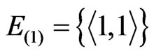
  be the set of directed edges between two nodes. A software mirror graph is a directed graph with a set of attributes
  being defined as follows:
 the number of times method i and method j are consecutively executed,
 the minimal number of steps (transitions) from an execution of method i to an execution of method j,
 .
.
The software mirror graph can be denoted  . Note that
  represents the temporal distance from node i to node j. Further,
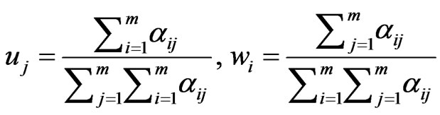
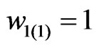
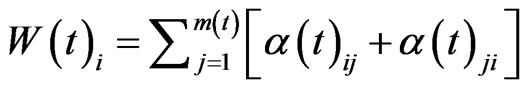
  represents the in vertex weight degree of node j, and thus
  represents the relative frequency of that an arbitrary method and method j are consecutively executed. Similarly,
  represents the out vertex weight degree of node i, and thus
  represents the relative frequency of that method i and an arbitrary method are consecutively executed.
Software mirror graph evolves as the software execution trace proceeds. Note that methods are visited and executed one by one, and thus the time domain for the software execution process should be discrete. Denote the software mirror graph at time t as .
.
It represents the software state at time t and looks like a mirror of the software state at time t.
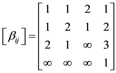
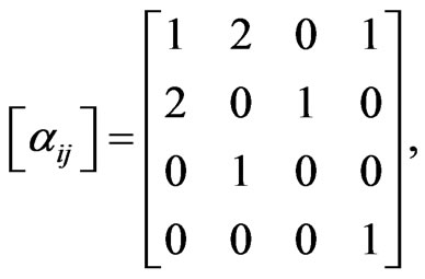
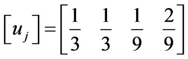
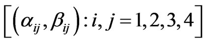
Let us take the execution trace of Figure 1 as an illustrative example.
There are four methods and thus . The total number of transitions of methods is 9, including the one method 1 is executed for the first time (from the initialization of the execution trace). We assume that the first execution of method 1 exactly follows a previous (virtual) execution of method 1. In this way
 . The corresponding attributes can be represented in the form of matrix as follows:
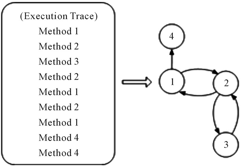
Figure 1. An execution trace and its directed topological graph.
 ,
, 
Now let us examine how a software mirror graph evolves as the software execution trace proceeds. Note that methods are visited and executed one by one, and thus the time domain for the software execution process should be discrete. Denote the software mirror graph at time t as . It represents the software state at time t and a snapshot of the software execution process. At the beginning of the software execution process or
 , only one method is executed and thus the software mirror graph contains only one node and one virtual edge (loop). For the execution trace of Figure 1, it holds that
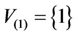 ,
,  ,
,  and
and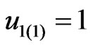 . At time
  a second method is executed, which may be or may not be the same one executed at time
 . A new node may or may not be added. A new edge may or may not be created. However the associated attributes must be assigned or updated. This results in an updated software mirror graph. More specifically, for the execution traceof Figure 1,
 of the software mirror graph evolves as follows:
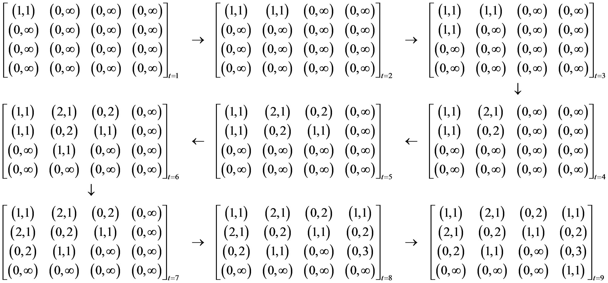
where as  evolves as follows:
and  evolves as follows:
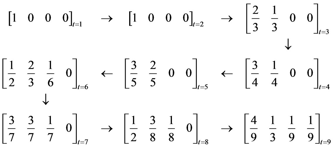
Note that  at time t means that there is no directed path from node i to node j up to time t. This simultaneously implies that
  at time t. Further,
  if and only if
 .
.
 is a graph that looks like a mirror of the software state at time t. The difference between a software mirror graph and a weighted topological graph can be clarified as follows. First, no self-loop may appear in a weighted topological graph. This is not the case for a software mirror graph and can be observed at time t = 9 for the execution trace of Figure 1. A selfloop appears if a method is consecutively executed twice. Second, only a single numerical attribute, whose physical interpretation is often obscure, is associated with each edge in a weighted topological graph. However in a software mirror graph, a set of attributes A is adopted to convey the dynamic information of interest with clear physical interpretations. The resulting software mirror graph evolves in the spatial dimension in terms of the nodes and edges as well as in the temporal dimension in terms of the dynamic attributes. Finally, the set of attributes A can be tailored or expanded if other static or dynamic information of the software execution process is of interest.
2.2.1. Degree Distribution
The degree of a node is defined as the number of edges connected to it. Degree distribution  is the probability that a node chosen uniformly at random has degree k, that is,
  is the fraction of nodes in the network that have degree k. For a directed topological graph, node i has in-degree
  as well as out-degree
 , which are defined as the number of ingoing edges to it and the number of outgoing edges from it, respectively.
The in-degree distribution describes the probabilities of  taking various values over the interval
 , and out-degree distribution describes the probabilities of
  taking various values over the interval
 . More specifically, the in-degree distribution and out-degree distribution are defined as
  and
and  respectively.
The cumulative in-degree distribution and out-degree distribution are defined as  and
and 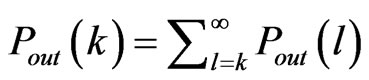 respectively.
Suppose that  follows a power law
 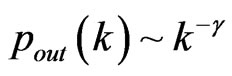 , then it holds
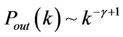 .
.
2.2.2. Vertex Weight Distribution
The definition of vertex weight distribution is similar to the definition of degree distribution. The difference is that the degree is replaced by the vertex weight which can be represented by  in the attribute set A.
The in vertex weight and out vertex weight are defined as:
 and
and  respectively. s here denotes the sum of weight of the each node.
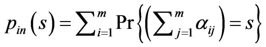
2.2.3. Average Path Length
The distance  from node i to node j in a software mirror graph with n nodes is defined as the number of edges on the shortest path from nodes i to node j.
 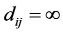 if there is no directed path from node i to node j. It is assumed that
  if
if . The average path length L of a mirror graph is then defined as follows:
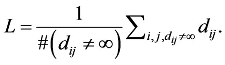
where 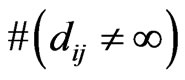 denotes the number of distances which are finite.
Here we note that besides the average path length, average temporal distance was also defined in our previous work [10]. It is defined to measure how many steps are required from an arbitrary method to another arbitrary method on average, which is calculated by the second attribute  in the attribute set A. In this paper, only the average path length is discussed as a traditional measure of the length of the network.
2.2.4. Clustering Coefficient
Clustering coefficient measures the conditional probability that an arbitrary triple of nodes defines a triangular of nodes (a third pair of topological neighbor) if the three nodes define two pairs of topological neighbors already [9]. Thus the clustering coefficient C is:
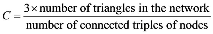 Here a triple of nodes is said to be connected if at least one of the three nodes takes the other two nodes as its topological neighbors. Note that clustering coefficient is only defined for undirected topological graphs. So in a directed one, two nodes are considered to be in neighbor if there is an edge from node i to node j, or vice versa.
2.3. Properties of the Software Mirror Graph
Three large-scale open-source GUI software systems were used in this paper as subject programs, including a tool kit for developing interactive 3D graphic applications named Intra3D, a tabbed browser with a customizable interface based on the Internet explorer browser engine named MyIE, and a tool for creating flowcharts, diagrams or slide shows named Diagram Designer. The programs were instrumented in advance in order to record the execution traces of the corresponding subject program while they were executed. In order to run a subject program, a test suit comprising various test cases was required to represent the input domain of the subject program. A test case is a sequence of primitive actions applied to the GUI program under operation [10]. Related statistics of the software operation platform are tabulated in Table 1.
In our software experiments 40 trials were conducted for each subject program. This generated 40 sets of experimental results for each subject program. The mean and standard deviation were then analyzed. This was aimed to guarantee the statistical repeatability of the software experiments. In our software experiments, 200 of 2000 test cases in the test suite were executed in a single trial of software execution for Intra3D, and 100 of 1000 test cases in the test suites were each executed in a single trial of software execution for MyIE and Diagram Designer.
Table 2 tabulates the results of the above measures for the three subject programs, where L and C denote the average path length and the average clustering coefficient of the networks built by the execution traces of the 40 trials.  and
and  denote the average path length
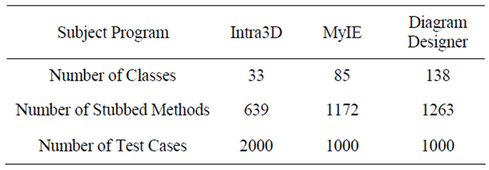
Table 1. Traces statistics of the three subject programs.
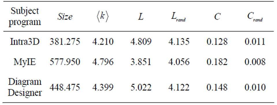
Table 2. Measures of the small-world effect.
and the clustering coefficient of a random graph of the same size and degree. It can be seen that L is comparable to , whereas C is much higher than
 . This means that the topological structure of the software execution processes demonstrate the small-world effects. In other words, the software execution process can be treated as a small-world network.
The out-degree distributions and the out-degree vertex weight distributions of the networks are showed in Figures 2 and 3. We can find that the curves in the loglog plot roughly fit a piecewise power law. This coincides with the observation presented in reference [10] that the out-degree distribution may be better treated as a piecewise power law than a single power law. Note here that a piecewise power law distribution is also a reflection of the scale-free property. However, it is less heterogeneous than a power law one because the proportion of nodes with high degree in the network of the former decreases.
3. The Proposed Model
3.1. The Generating Mechanisms of the Model
An evolving model is proposed in this paper to explain the formalization of the software mirror graph. The model should be capable of capturing the essential mechanisms responsible for the small-world effect and scale-free property. We analyze the characteristics of the execution process in the first place. First, the increment speed of the nodes in the network slows down with time and the number of nodes gradually tends to the total number of the methods in the software program. Second, the link among methods should obey the program logic, instead of attaching randomly among the whole network just like most of other real complex networks. After the program coding, the candidate methods that a method
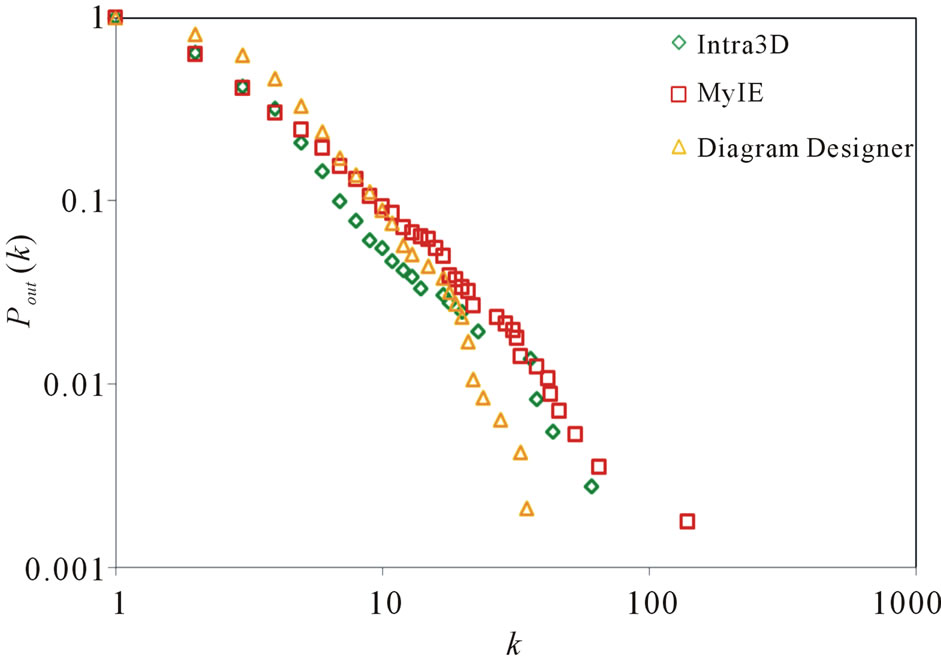
Figure 2. Out degree distribution.
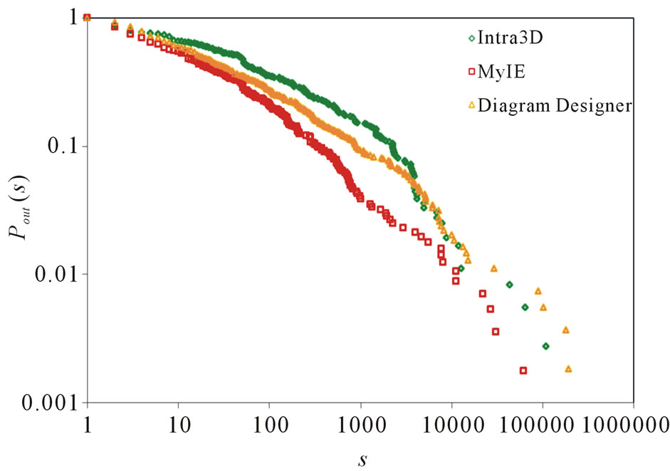
Figure 3. Vertex weight distribution.
can reach is fixed. Finally, uncertainty is associated with the software execution process, which stems from the uncertainty of execution profile, execution environment, and program multithreading, etc. Bugs in the program can also cause uncertainty to the execution process. Based on the analysis, we proposed a model which postulates that there are three fundamental mechanisms: growth, preferential attachment, and walking on the network. The model is described as follows:
Step 1: Growth: Starting with a small number  of nodes
  and a small number
  of edges at time t0. The weight on each edge is set to be one. Constant N is given to represent the total number of nodes, and S the total weight of the edges. At each time step from t1, a new node
  is added with probability
 , where
  denotes the number of nodes at time
 , and a is a constant ranged
 .
.
Step 2: Preferential attachment: At each time step from t1, select a node  from the network with probability p2, which is a constant ranged
 . If this action is taken, the probability of node i to be selected is proportional to
 , where
 ,
,  is the number of the neighbors of node i at time t, and
  denotes the weight of the edge from node i to node j. Note here
  , where
  is the number of nodes at time
 .
.
Select a node  from the network. The probability of node i to be selected is proportional to
 , where
  ,
,  is the number of the neighbors of node i at time t, and
  denotes the weight of the edge from node i to node j.
If both of  and
and  exist, then link
  to
to , and
, and  to
to . If only one of the two exists, then link the one to
 . The corresponding weight on each edge adds one at the same time.
Step 3: Walk along the neighborhood: Set  to be the current node, from the current node, walk in the network according to the following rule:
Select a node in the neighborhood of the current node. The probability of a node i in the neighborhood to be selected is proportional to , where
 ,
,  is the number of the neighbors of node i at time t, and
  denotes the weight of the edge from node i to node j. Note here
  and
and , where
  is the number of nodes at time t.
Link an edge from the current node to the selected node if the edge is absent. And the corresponding weight on the edge added one at the same time. The total weight  at time t added one simultaneously. Note here
  is initially set to be zero at the beginning of this step.
Set the selected node to be the current node. If  equals to a constant e, stop this step. Else continue walking in its neighborhood according to the rule described above.
Step 4: If  equals to a constant S, stop the process. Otherwise, go to Step 1. Note here Weight is initially set to be zero at the beginning of the process.
3.2. The Simulation Results of the Modle
In this section, we give the simulation results of the proposed model, and discuss the relationship of parameters setting and the network properties.
3.2.1. The Total Node Number N
Set ,
,  ,
,  ,
, . Figure 4 gives the out degree distribution, out vertex weight degree distribution, average path length and clustering coefficient while N takes 100, 200, 500 and 1000 respectively. From Figure 4 we can see that the distributions of the out degree and the out vertex weight degree roughly fit a piecewise power law. Along with the increase of N, the power exponent k of the first stage increases, while that of the second stage decreases, which makes the curve more and more fit a power law. Along with the increases of N, the average path length increases and the clustering coefficient decreases. However, the average path length keeps short and the coefficient keeps small, which means the world is still small although it turns a little bigger with the network growing.
3.2.2. Parameter a
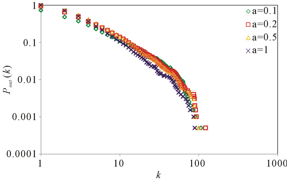
If N is set, parameter a decides the probability to introduce a new node into the network. Set ,
,  ,
,  ,
, . Figure 5 gives the out degree distribution, out vertex weight degree distribution, average path length and clustering coefficient while a takes 0.1, 0.2, 0.5 and 1 respectively. From Figure 5 we can see that the influence of parameter a is not obvious. Along with the increase of a, the average path length increases slightly and the clustering coefficient decreases slightly, which means the world is still small although it turns a little bigger.
3.2.3. Probability p2
p2 decides the probability of preferentially attaching a node which already exists in the network before choosing a node to be the start point of walking. Set ,
,  ,
,  ,
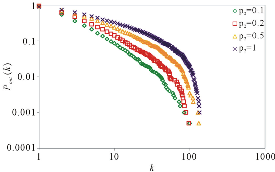
, . Figure 6 gives the out degree distribution, out vertex weight degree distribution, average path length and clustering coefficient while p2 takes 0.1, 0.2, 0.5 and 1 respectively. Figure 6 shows that along with the increase of p2, the heterogeneity gets worse and the curve fits more and more like a piecewise power law. However, the influence of p2 on the vertex weight degree distribution is not obvious. Along with the increase of p2, the average path length decreases slightly and the clustering coefficient increases slightly, which means the world gets a little smaller.
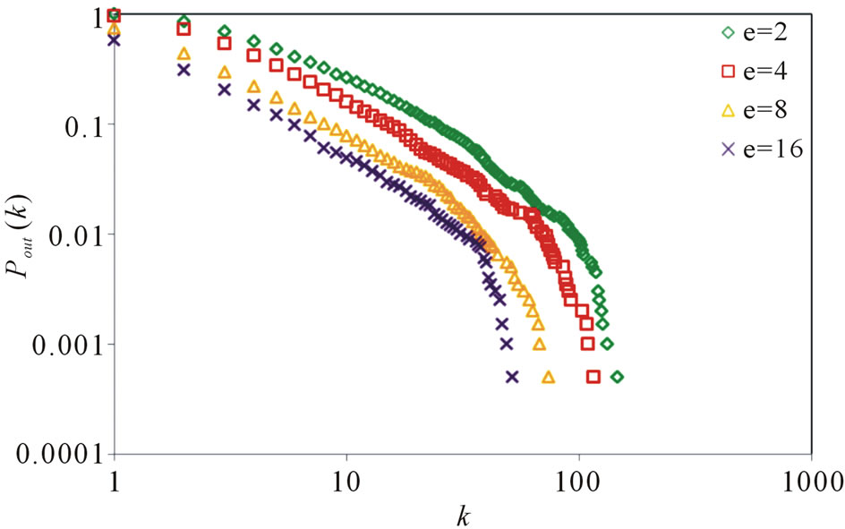
3.2.4. The Total Weight e Added in Each Time Step
e decides the the total weight to be added in each time step. Set ,
,  ,
, . Figure 7 gives the out degree distribution, out vertex weight degree distribution, average path length and clustering coefficient while e takes 2, 4, 8 and 16 respectively. Figure 7 shows that e does not change the power exponent of the piecewise power law. However, it makes the curve moves parallelly to the left. From Figure 7 we can see that along with the increase of e, the average path length increases slightly and the clustering coefficient decreases slightly, which means the world is still small although it
 (a)
(a) (b)
(b) (c)
(c) (d)
(d)
Figure 4. a = 0.2, p2 = 0.2, e = 5, S = 100,000.
 (a)
(a)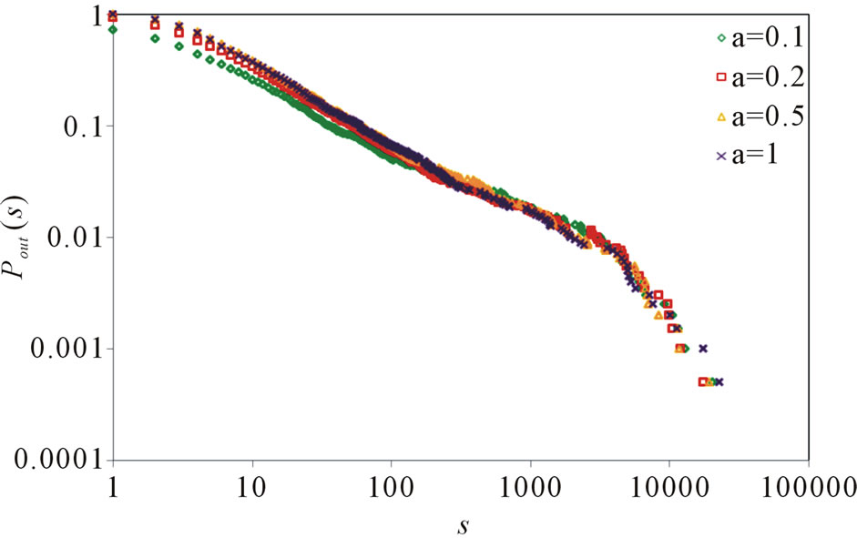 (b)
(b)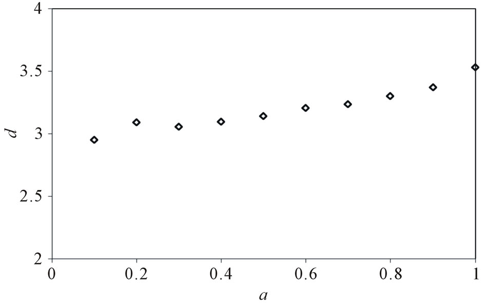 (c)
(c)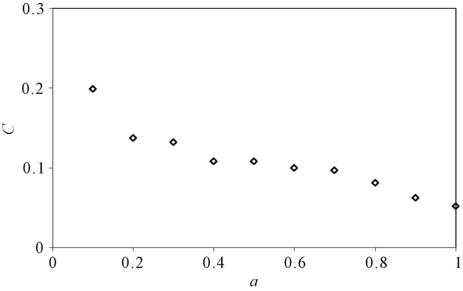 (d)
(d)
Figure 5. N = 500, p2 = 0.2, e = 5, S = 100,000.
 (a)
(a)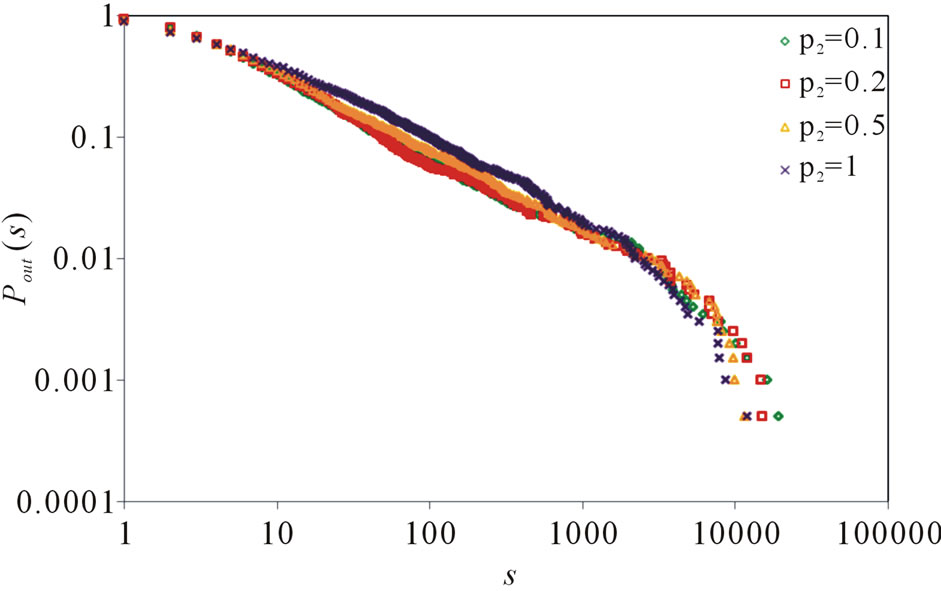 (b)
(b)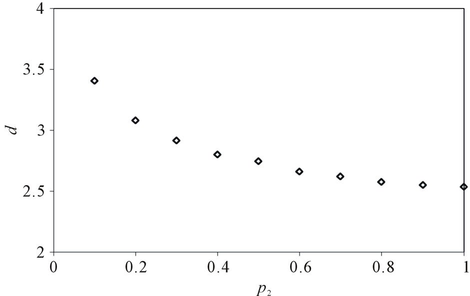 (c)
(c)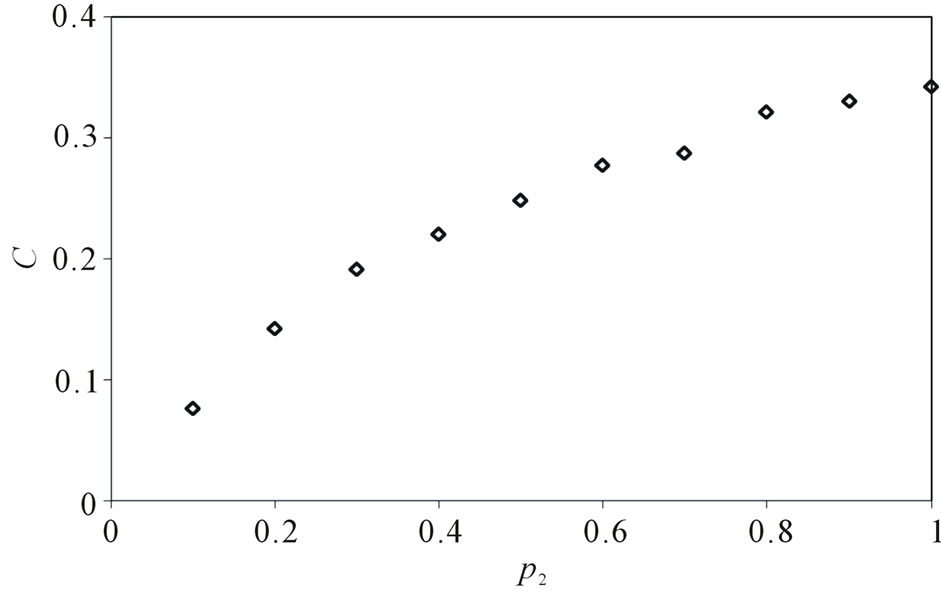 (d)
(d)
Figure 6. N = 500, a = 0.2, e = 5, S = 100,000.
 (a)
(a)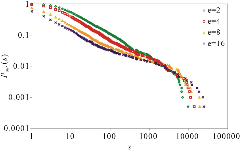 (b)
(b)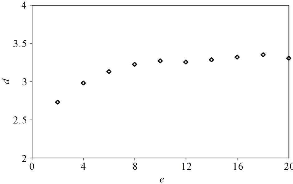 (c)
(c)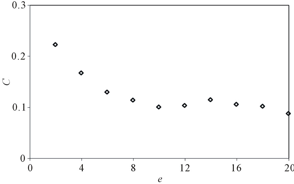 (d)
(d)
Figure 7. N = 500, a = 0.2, p2 = 0.2, S = 100,000.
turns a little bigger.
3.3. Discussion
The model and the simulation results are further discussed here. In Part 2 of Section 3 we analyzed the characteristic of the execution process. In brief, the number of executed methods goes stable with time, and the methods are executed according to the program logic with some elements of uncertainty. In the model proposed in Part 1 of Section 3, we can see that the probability of introducing a new node is proportional to , which keeps decreasing along with time. When
  increases up to N, the number of the nodes in the network stops increasing and the evolving of the network only reflect by the increasing of edges or weights. The dynamic execution process can be treated as walking along the software static structure according to the execution profile, so instead of linking randomly, the node can only link its neighbors in the static structure. The topology of the execution process network can be treated as a union set of a lot of sub graphs of the software static structure and the repetitive edges are represented by weight on the edge. The uncertainty in the model is reflected in three ways: the selection of the start node
  of the walking in each time step, the selection of
  which bridge the new added node
  and
and , and the selection of the nodes on the walking route.
From the simulation results, we can see that the model generates a network being both scale-free and small world. The trend of the curves consists with that of the real software system. Along with the increase of N and decrease of p2, the topological network turns more and more scale-free, and the curve fits more like a power law. The parameter e only has influence on the turning point, and makes it move to the left along with e increasing. The scale-free property of the execution process network first comes from static structure of the software program which has been widely reported to be scale-free. The reuse of basic functions and the decomposition of main functions make the “hubs” emerge in the network and lead to the scale-free property. While executed, these hubs naturally have more chances to be selected. The preferential attachment is another cause of the scale-free property, due to the execution profile, some functions are executed with a higher probability, which makes the corresponding methods possesses more edges or weight.
The parameters all have influence on the short path length and clustering coefficient. However, the network keeps being a small world. We can notice that the parameter p2 make the network to be even smaller with its increasing. It is not hard to be understood because p2 decides the probability to add  which can provide “long-distance” connections in the network.
4. Conclusions
In recent years a number of related works treated software systems as complex networks and found that software systems might also be small world and follow scale-free degree distributions. Our previous work [10] revealed that not only the software static structure, but also the networks of software dynamic execution processes (software mirror graph) may have small world effect and scale-free property. Up to now, there exist no wild accepted models that can describe the mechanisms that generate the small world and scale-free software networks.
In this paper, we first reviewed the software mirror graph of the software execution process. And then we gave the definitions of the network measures and properties. The experimental results of three real software were presented and showed the networks are scale-free and small world. Then an evolving model was proposed based on the analysis of the execution process. The model has three basic mechanisms: growth, preferential attachment, and walking in the neighborhood. The model can well describe the evolving process and the simulation results showed that it can reflect the network properties. The influence of parameters was then discussed and we found the number of nodes in network and the probability p2 of adding the bridge nodes affected the scale-free property. And p2 also affects the small-world effect which makes the world turning to be even smaller with its increase.
A possible work we can do in future is to examine more subject programs to find the network properties of their execution process. Moreover, based on the proposed model, we may carry out research on software bug localization because as what we discussed in previous sections, bugs causes uncertainty and may change the network structure and properties.
5. Acknowledgements
This work is supported by the National Science Foundation of China under Grant No. 60973006, and the Beijing Natural Science Foundation under Grant No. 4112033.
REFERENCES
- A. de Moura, Y.-C. Lai and A. Motter, “Signatures of Small-World and Scale-Free Properties in Large Computer Programs,” Physical Reviews E, Vol. 68, 2003.
- S. Valverde, R. Ferrer-Cancho and R. Sole, “Hierarchical Small Worlds in Software Architecture,” Santa Fe Institute Working Papers, SFI/03-07-044, 2003.
- A. Gorshenev and Y. Pis’mak, “Punctuated Equilibrium in Software Evolution,” Physical Reviews E, Vol. 70, 2004.
- A. Potanin, J. Noble, M. Frean and R. Biddle, “Scale-Free Geometry in Object-Oriented Programs,” Communication of the ACM, Vol. 48, No. 5, 2005, pp. 99-103. doi:10.1145/1060710.1060716
- S. Jenkins and S. R. Kirk, “Software Architecture Graphs as Complex Networks: A Novel Partitioning Scheme to Measure Stability and Evolution,” Information Sciences, Vol. 177, No. 5, 2007, pp. 2587-2601. doi:10.1016/j.ins.2007.01.021
- G. Concas, M. Marchesi, S. Pinna and N. Serra, “PowerLaws in a Large Object-Oriented Software System,” IEEE Transactions on Software Engineering, Vol. 33, No. 10, 2007, pp. 687-707. doi:10.1109/TSE.2007.1019
- P. Louridas, D. Spinellis and V. Vlachos, “Power Laws in Software,” ACM Transactions on Software Engineering and Methodology, Vol. 18, No. 1, 2008, pp. 1-26. doi:10.1145/1391984.1391986
- L. Hatton, “Power-law Distributions of Component Size in General Software Systems,” IEEE Transactions on Software Engineering, Vol. 35, No. 4, 2009, pp. 566-572. doi:10.1109/TSE.2008.105
- M. E. J. Newman, “The Structure and Function of Complex Networks,” SIAM Review, Vol. 45, No. 2, 2003, pp. 167-256. doi:10.1137/S003614450342480
- K. Y. Cai and B. B. Yin, “Software Execution Processes as an Evolving Complex Network,” Information Sciences, Vol. 179, No. 12, 2009, pp. 1903-1928. doi:10.1016/j.ins.2009.01.011
- D. J. Watts and S. H. Strogatz, “Collective Dynamics of ‘Small-World’ Networks,” Nature, Vol. 393, 1998, pp. 440- 442. doi:10.1038/30918
- A.-L. Barabási and R. Albert, “Emergence of Scaling in Random Networks,” Science, Vol. 286, No. 5439, 1999, pp. 509-512. doi:10.1126/science.286.5439.509
- S. Valverde, R. Ferror Cancho and R. V. Sole, “ScaleFree Networks from Optimal Design,” cond-mat/0204344, April 2002.
- C. Myers, “Software Systems as Complex Networks: Structure, Function, and Evolvability of Software Collaboration Graphs,” Physical Reviews E, Vol. 68, 2003.
- S. Valverde and R. Sole, “Network Motifs in Computational Graphs: A Case Study in Software Architecture,” Physical Review E, Vol. 72, No. 2, 2005, Article ID: 026107.
- K. He, R. Peng, J. Liu, F. He, et al., “Design Methodology of Networked Software Evolution Growth Based on Software Patterns,” Journal of System Science and Complexity, Vol. 19, No. 2, 2006, pp. 157-181. doi:10.1007/s11424-006-0157-6