Applied Mathematics
Vol.06 No.08(2015), Article ID:58451,17 pages
10.4236/am.2015.68131
Formulation of a Preconditioned Algorithm for the Conjugate Gradient Squared Method in Accordance with Its Logical Structure
Shoji Itoh1, Masaaki Sugihara2
1Division of Science, School of Science and Engineering, Tokyo Denki University, Saitama, Japan
2Department of Physics and Mathematics, College of Science and Engineering, Aoyama Gakuin University, Kanagawa, Japan
Email: itosho@acm.org
Copyright © 2015 by authors and Scientific Research Publishing Inc.
This work is licensed under the Creative Commons Attribution-NonCommercial International License (CC BY-NC).
http://creativecommons.org/licenses/by-nc/4.0/


Received 22 June 2015; accepted 27 July 2015; published 30 July 2015
ABSTRACT
In this paper, we propose an improved preconditioned algorithm for the conjugate gradient squared method (improved PCGS) for the solution of linear equations. Further, the logical structures underlying the formation of this preconditioned algorithm are demonstrated via a number of theorems. This improved PCGS algorithm retains some mathematical properties that are associated with the CGS derivation from the bi-conjugate gradient method under a non-preconditioned system. A series of numerical comparisons with the conventional PCGS illustrate the enhanced effectiveness of our improved scheme with a variety of preconditioners. This logical structure underlying the formation of the improved PCGS brings a spillover effect from various bi-Lanczos-type algorithms with minimal residual operations, because these algorithms were constructed by adopting the idea behind the derivation of CGS. These bi-Lanczos-type algorithms are very important because they are often adopted to solve the systems of linear equations that arise from large-scale numerical simulations.
Keywords:
Linear Systems, Krylov Subspace Method, Bi-Lanczos Algorithm, Preconditioned System, PCGS

1. Introduction
In scientific and technical computation, natural phenomena or engineering problems are described through numerical models. These models are often reduced to a system of linear equations:
 (1)
(1)
where A is a large, sparse coefficient matrix of size ,
,
 is the solution vector, and
 is the right-hand side (RHS) vector.
The conjugate gradient squared (CGS) method is a way to solve (1) [1] . The CGS method is a type of bi- Lanczos algorithm that belongs to the class of Krylov subspace methods.
Bi-Lanczos-type algorithms are derived from the bi-conjugate gradient (BiCG) method [2] [3] , which assumes the existence of a dual system
 (2)
(2)
Characteristically, the coefficient matrix of (2) is the transpose of A. In this paper, we term (2) a “shadow system”.
Bi-Lanczos-type algorithms have the advantage of requiring less memory than Arnoldi-type algorithms, another class of Krylov subspace methods.
The CGS method is derived from BiCG. Furthermore, various bi-Lanczos-type algorithms, such as BiCGStab [4] , GPBiCG [5] and so on, have been constructed by adopting the idea behind the derivation of CGS. These bi-Lanczos-type algorithms are very important because they are often adopted to solve systems in the form of (1) that arise from large-scale numerical simulations.
Many iterative methods, including bi-Lanczos algorithms, are often applied together with some preconditioning operation. Such algorithms are called preconditioned algorithms; for example, preconditioned CGS (PCGS). The application of preconditioning operations to iterative methods effectively enhances their performance. Indeed, the effects attributable to different preconditioning operations are greater than those produced by different iterative methods [6] . However, if a preconditioned algorithm is poorly designed, there may be no beneficial effect from the preconditioning operation.
Consequently, PCGS holds an important position within the Krylov subspace methods. In this paper, we identify a mathematical issue with the conventional PCGS algorithm, and propose an improved PCGS1. This improved PCGS algorithm is derived rationally in accordance with its logical structure.
In this paper, preconditioned algorithm and preconditioned system refer to solving algorithms described with some preconditioning operator M (or preconditioner, preconditioning matrix) and the system converted by the operator based on M, respectively. These terms never indicate the algorithm for the preconditioning operation itself, such as “incomplete LU decomposition”, “approximate inverse”, and so on. For example, for a preconditioned system, the original linear system (1) becomes
![]() (3)
(3)
![]() (4)
(4)
under the preconditioner
![]()
![]() . Here, the matrix and the vector in the preconditioned system are denoted by the tilde
. Here, the matrix and the vector in the preconditioned system are denoted by the tilde![]() . However, the conversions in (3) and (4) are not implemented; rather, we construct the preconditioned algorithm that is equivalent to solving (3).
. However, the conversions in (3) and (4) are not implemented; rather, we construct the preconditioned algorithm that is equivalent to solving (3).
This paper is organized as follows. Section 2 provides an overview of the derivation of the CGS method and the properties of two scalar coefficients (![]() and
and![]() ). This forms an important part of our argument for the preconditioned BiCG and PCGS algorithms in the next section. Section 3 introduces the PCGS algorithm. An issue with the conventional PCGS algorithm is identified, and an improved algorithm is proposed. In Section 4, we present some numerical results to demonstrate the effect of the improved PCGS algorithm with a variety of preconditioners. As a consequence, the effectiveness of the improved algorithm is clearly established. Finally, our conclusions are presented in Section 5.
). This forms an important part of our argument for the preconditioned BiCG and PCGS algorithms in the next section. Section 3 introduces the PCGS algorithm. An issue with the conventional PCGS algorithm is identified, and an improved algorithm is proposed. In Section 4, we present some numerical results to demonstrate the effect of the improved PCGS algorithm with a variety of preconditioners. As a consequence, the effectiveness of the improved algorithm is clearly established. Finally, our conclusions are presented in Section 5.
2. Derivation of the CGS Method and Preconditioned Algorithm of the BiCG Method
In this section, we derive the CGS method from the BiCG method, and introduce the preconditioned BiCG algorithm.
2.1. Structure of the BiCG Method
BiCG [2] [3] is an iterative method for linear systems in which the coefficient matrix A is nonsymmetric. The algorithm proceeds as follows:
Algorithm 1. BiCG method:
![]() is an initial guess,
is an initial guess,
![]() , set
, set ,
,
 , e.g.,
For
 until convergence, Do:

 (5)
(5)


 (6)
(6)
End Do
BiCG implements the following Theorems.
Theorem 1 (Hestenes et al. [8] , Sonneveld [1] , and others.)2 For a non-preconditioned system, there are recurrence relations that define the degree k of the residual polynomial
 and probing direction polynomial
 . These are
 (7)
(7)
 (8)
(8)
 (9)
(9)
where
 and
and
 are based on (5) and (6).
Using the polynomials of Theorem 1, the residual vector for the linear system (1) and the shadow residual vector for the shadow system (2) can be written as
 (10)
(10)
 (11)
(11)
These probing direction vectors are represented by
 (12)
(12)
 (13)
(13)
where
 is the initial residual vector and
 is the initial shadow residual vector. However, in practice,
 is set in such a way as to satisfy the conditions
 .
.
 denotes the inner product between vectors u and
 . In this paper, we set
 to satisfy the conditions
 exactly. This is a typical way of ensuring
 ; other settings are beyond the scope of this paper.
Theorem 2 (Fletcher [2] ) The BiCG method satisfies the following conditions:
 (14)
(14)
 (15)
(15)
2.2. Derivation of the CGS Method
The CGS method is derived by transforming the scalar coefficients in the BiCG method to avoid the
 matrix [1] . The polynomial defined by (10)-(13) is substituted into (14) and (15), which construct the numerator and denominator of
 and
and
 in BiCG3. Then,
 (16)
(16)
 (17)
(17)
and the following theorem can be applied.
Theorem 3 (Sonneveld [1] ) The CGS coefficients
 and
and
 are equivalent to these coefficients in BiCG under certain transformation and substitution operations based on the bi-orthogonality and bi-conjugacy conditions.
Proof. We apply
 (18)
(18)
to (16) and (17). Then,
 (19)
(19)
 (20)
(20)
□
The CGS method is derived from BiCG by Theorem 4.

3In this paper, if we specifically distinguish this algorithm, we write
 and
and .
.
4In this paper, we use the superscript “CGS” alongside ,
,
 , and relevant vectors to describe this algorithm.
Theorem 4 (Sonneveld [1] ) The CGS method is derived from the linear system’s recurrence relations in the BiCG method under the property of equivalence between the coefficients ,
,
 in CGS and BiCG. However,
the solution vector
 is derived from a recurrence relation based on
 .
.
Proof. The coefficients
 and
and
 in BiCG and CGS were derived in Theorem 3. The recurrence relations (8) and (9) for BiCG are squared to give:
 (21)
(21)
 (22)
(22)
Further, we can apply ,
,
 from (18), and substitute
 ,
, . □
. □
Thus, we have derived the CGS method4.
Algorithm 2. CGS method:
 is an initial guess,
 set
set

 , e.g.,
For
 until convergence, Do:


End Do
The following Proposition 5 and Corollary 1 are given as a supplementary explanation for Algorithm 2. These are almost trivial, but are comparatively important in the next section’s discussion.
Proposition 5 There exist the following relations:
 (23)
(23)
 (24)
(24)
where
 is the initial residual vector at
 in the iterative part of CGS,
 is the initial shadow residual vector in CGS,
 is the initial residual vector, and
 is the initial shadow residual vector.
Proof. Equation (23) follows because (18) for
 gives
gives![]() . Here,
. Here,
![]() by (7), and I denotes the identity matrix.
by (7), and I denotes the identity matrix.
Equation (24) is derived as follows. Applying (18) to (16), we obtain
![]()
This equation shows that the inner product of the CGS on the right is obtained from the inner product of the BiCG on the left. Therefore,
![]() that composes the polynomial
that composes the polynomial
![]() to express the shadow residual vector of the BiCG is the same as
to express the shadow residual vector of the BiCG is the same as
![]() in CGS.
in CGS.
Hereafter,
![]() can be represented by
can be represented by![]() , to the extent that neither can be distinguished. □
, to the extent that neither can be distinguished. □
Corollary 1. There exists the following relation:
![]()
where
![]() is the probing direction vector in CGS,
is the probing direction vector in CGS,
![]() is the initial residual vector at
is the initial residual vector at
![]() in the iterative part of CGS, and
in the iterative part of CGS, and
![]() is the initial residual vector.
is the initial residual vector.
2.3. Derivation of Preconditioned BiCG Algorithm
In this subsection, the preconditioned BiCG algorithm is derived from the non-preconditioned BiCG method (Algorithm 1). First, some basic aspects of the BiCG method under a preconditioned system are expressed, and a standard preconditioned BiCG algorithm is given.
When the BiCG method (Algorithm 1) is applied to linear equations under a preconditioned system:
![]() (25)
(25)
we obtain a “BiCG method under a preconditioned system” (Algorithm 3). We denote this as “PBiCG”.
In this paper, matrices and vectors under the preconditioned system are denoted with “![]() ”, such as
”, such as![]() ,
,
![]() 5. The coefficients
5. The coefficients![]() ,
,
![]() are specified by
are specified by![]() ,
,![]() .
.
Algorithm 3. BiCG method under the preconditioned system:
![]() is an initial guess,
is an initial guess,
![]() , set
, set![]() ,
,
![]() , e.g.,
, e.g.,
For
![]() until convergence, Do:
until convergence, Do:
![]()
![]() (26)
(26)
![]()
![]()
![]() (27)
(27)
End Do
![]()
5If we wish to emphasize different methods, a superscript is applied to the relevant vectors to denote the method, such as![]() ,
,![]() .
.
6We represent the polynomials R and P in italic font to denote a preconditioned system.
We now state Theorem 6 and Theorem 7, which are clearly derived from Theorem 1 and Theorem 2, respectively.
Theorem 6. Under the preconditioned system, there are recurrence relations that define the degree k of the residual polynomial
![]() and probing direction polynomial
and probing direction polynomial
![]() 6. These are
6. These are
![]() (28)
(28)
![]() (29)
(29)
![]() (30)
(30)
where
![]() is the variation under the preconditioned system, and
is the variation under the preconditioned system, and![]() ,
,
![]() in these relations are based on (26) and (27).
in these relations are based on (26) and (27).
Using the polynomials of Theorem 6, the residual vectors of the preconditioned linear system (25) and the shadow residual vectors of the following preconditioned shadow system:
![]() (31)
(31)
can be represented as
![]() (32)
(32)
![]() (33)
(33)
respectively. The probing direction vectors are given by
![]() (34)
(34)
![]() (35)
(35)
respectively. Under the preconditioned system,
![]() is set in such a way as to satisfy the conditions
is set in such a way as to satisfy the conditions![]() . In this paper, we set
. In this paper, we set
![]() based on the equation
based on the equation
![]() to satisfy the conditions
to satisfy the conditions
![]() exactly. Some variations based on
exactly. Some variations based on![]() , such as Algorithm 4 below, are allowed. Other settings are beyond the scope of this paper.
, such as Algorithm 4 below, are allowed. Other settings are beyond the scope of this paper.
Remark 1. The shadow systems given by (31) do not exist, but it is very important to construct systems in which the transpose of the matrix
![]() exists.
exists.
Theorem 7. The BiCG method under the preconditioned system satisfies the following conditions:
![]() (36)
(36)
![]() (37)
(37)
Next, we derive the standard PBiCG algorithm. Here, the preconditioned linear system (25) and its shadow system (31) are formed as follows:
![]() (38)
(38)
![]() (39)
(39)
Definition 1. On the subject of the PBiCG algorithm, the solution vector is denoted as![]() . Furthermore, the residual vectors of the linear system and shadow system of the PBiCG algorithm are written as
. Furthermore, the residual vectors of the linear system and shadow system of the PBiCG algorithm are written as
![]() and
and![]() , respectively, and their probing direction vectors are
, respectively, and their probing direction vectors are
![]() and
and![]() , respectively.
, respectively.
Using this notation, each vector of the BiCG under the preconditioned system given by Algorithm 3 is converted as below:
![]() (40)
(40)
Substituting the elements of (40) into (36) and (37), we have
![]() (41)
(41)
![]() (42)
(42)
Consequently, (26) and (27) become
![]() (43)
(43)
![]() (44)
(44)
Before the iterative step, we give the following Definition 2.
Definition 2. For some preconditioned algorithms, the initial residual vector of the linear system is written as
![]() and the initial shadow residual vector of the shadow system is written as
and the initial shadow residual vector of the shadow system is written as
![]() before the iterative step.
before the iterative step.
We adopt the following preconditioning conversion after (40).
![]() (45)
(45)
Consequently, we can derive the following standard PBiCG algorithm [9] [10] .
Algorithm 4. Standard preconditioned BiCG algorithm:
![]() is an initial guess,
is an initial guess,
![]() set
set![]() ,
,
![]() , e.g.,
, e.g.,
For
![]() until convergence, Do:
until convergence, Do:
![]()
![]()
![]() (46)
(46)
![]()
![]() (47)
(47)
![]() (48)
(48)
![]() (49)
(49)
End Do
Algorithm 4 satisfies
![]() and
and
![]() when
when
![]() in the iterative part.
in the iterative part.
Remark 2. Because we apply a preconditioning conversion such as
![]() in the iteration of the BiCG method under the preconditioned system (Algorithm 3),
in the iteration of the BiCG method under the preconditioned system (Algorithm 3),
![]() when
when
![]() in the iteration of Algorithm 4. Further, the initial solution to Algorithm 3 is technically
in the iteration of Algorithm 4. Further, the initial solution to Algorithm 3 is technically![]() , but this is actually calculated by multiplying
, but this is actually calculated by multiplying
![]() by the initial solution
by the initial solution![]() .
.
In this section, we have shown that
![]() in BiCG is equivalent to
in BiCG is equivalent to
![]() in CGS using (19), and that
in CGS using (19), and that
![]() in BiCG is equivalent to
in BiCG is equivalent to
![]() in CGS using (20). In the next section, we propose an improved PCGS algorithm by applying this result to the preconditioned system.
in CGS using (20). In the next section, we propose an improved PCGS algorithm by applying this result to the preconditioned system.
3. Improved PCGS Algorithm
In this section, we first explain the derivation of PCGS, and present the conventional PCGS algorithm. We identify an issue with this conventional PCGS algorithm, and propose an improved PCGS that overcomes this issue.
3.1. Derivation of PCGS Algorithm
Figure 1 illustrates the logical structure of the solving methods and preconditioned algorithms discussed in this paper.
![]()
Figure 1. Relation between BiCG, CGS, and their preconditioned algorithms.
Typically, PCGS algorithms are derived via a “CGS method under a preconditioned system” (Algorithm 5).
Algorithm 5 is derived by applying the CGS method (Algorithm 2) to the preconditioned linear system (25). In this section, the vectors and![]() ,
,
 are PCGS elements, except for those before the iteration (Definition 2). If we wish to emphasize different methods, we apply a superscript to the relevant vectors, such as
 ,
,
 ,
,
 ,
, .
.
Algorithm 5. CGS method under the preconditioned system:
 is an initial guess,
 , set
, set ,
,
 , e.g., ,
For
 until convergence, Do:


End Do
The conventional PCGS algorithm (Algorithm 6) is derived via the CGS method, as shown in Figure 1, but this algorithm does not reflect the logic of subsection 2.2 in its preconditioning conversion. In contrast, our proposed improved PCGS algorithm (Algorithm 7) directly applies the derivation from BiCG to CGS to the PBiCG algorithm, thus maintaining the logic from subsection 2.2.
3.2. Conventional PCGS and Its Issue
The conventional PCGS algorithm is adopted in many documents and numerical libraries [4] [9] [11] . It is derived by applying the following preconditioning conversion to Algorithm 5:
 (50)
(50)
This gives the following Algorithm 6 (“Conventional PCGS” in Figure 1).
Algorithm 6. Conventional PCGS algorithm:
 is an initial guess,
 ,
,
 , e.g.,
 set
set

For
 until convergence, Do:


 (51)
(51)


 (52)
(52)
End Do
This PCGS algorithm was described in [4] , which proposed the BiCGStab method, and has been employed as a standard approach as affairs stand now.
This version of PCGS seems to be a compliant algorithm on the surface, because the operation
 in (51) and (52) does not include the preconditioning operator
 under the conversions
 and
and
 from (50). However, if we apply
 from (50) to the preconditioning conversion of the shadow residual vector in the BiCG method, we obtain
 (53)
(53)
This is different to the conversion given by (40), and we cannot obtain equivalent coefficients to ,
,
 in (43) and (44) using (53).
3.3. Derivation of the CGS Method from PBiCG
In this subsection, we present an improved PCGS algorithm (“Improved PCGS” in Figure 1). We formulate this algorithm by applying the CGS derivation process to the BiCG method directly under the preconditioned system (PBiCG, Algorithm 3).
The polynomials (32)-(35) of the residual vectors and the probing direction vectors in PBiCG are substituted for the numerators and denominators of
 and
and . We have
 (54)
(54)
 (55)
(55)
and apply the following Theorem 8.
Theorem 8. The PCGS coefficients
 and
and
 are equivalent to these coefficients in PBiCG under certain transformation and substitution operations based on the bi-orthogonality and bi-conjugacy conditions under the preconditioned system.
Proof. We apply
 (56)
(56)
to (54) and (55). Then,
 (57)
(57)
 (58)
(58)
□
The PCGS method is derived from PBiCG using Theorem 9.
Theorem 9. The PCGS method is derived from the linear system’s recurrence relations in the PBiCG method under the property of equivalence between the coefficients ,
,
 in PCGS and PBiCG. However, the solution vector
 is derived from a recurrence relation based on
 .
.
Proof. The coefficients
 and
and
 in PBiCG and PCGS were derived in Theorem 8. The recurrence relations in (29) and (30) for PBiCG are squared to give:
 (59)
(59)
 (60)
(60)
Further, we can apply
 from (56), and substitute
 ,
, . □
. □
The following Proposition 10 and Corollary 2 are given as a supplementary explanation under the preconditioned system.
Proposition 10. There exist the following relations:
 (61)
(61)
 (62)
(62)
where
 is the initial residual vector at
 in the iterative part of PCGS,
 is the initial shadow residual vector in PCGS,
 is the initial residual vector, and
 is the initial shadow residual vector.
Proof. Equation (61) follows because (56) for
 gives
gives . Here,
 by (28).
Equation (62) is derived as follows. Applying (56) to (54), we obtain

This equation shows that the inner product of the PCGS on the right is obtained from the inner product of the PBiCG on the left. Therefore,
 that composes the polynomial
 to express the shadow residual vector of the PBiCG is the same as
 in PCGS.
Hereafter,
 can be represented by
 , to the extent that neither can be distinguished. □
Corollary 2. There exists the following relation:

where
 is the probing direction vector in PCGS,
 is the initial residual vector at
 in the iterative part of PCGS, and
 is the initial residual vector.
The CGS preconditioning conversion given by ,
,
 , and
, and
 is subjected to the same treatment as the BiCG preconditioning conversion of
 ,
,
 , in (40) and (45). Further,
 is the same as
 . Then,
 (63)
(63)
 (64)
(64)

7We apply the superscript “PCGS” to ,
,
 , and relevant vectors to denote this algorithm.
As a consequence, the following improved PCGS algorithm is derived7.
Algorithm 7. Improved preconditioned CGS algorithm:
 is an initial guess,
 ,
,
 , e.g.,
 set
set

For
 until convergence, Do:


End Do
Algorithm 7 can also be derived by applying the following preconditioning conversion to Algorithm 5. Here, we treat the preconditioning conversions of
 and
and
 the same as the conversion of
 .
.

The number of preconditioning operations in the iterative part of Algorithm 7 is the same as that in Algorithm 6.
4. Numerical Experiments
In this section, we compare the conventional and improved PCGS algorithms numerically.
The test problems were generated by building real unsymmetric matrices corresponding to linear systems taken from the Tim Davis collection [12] and the Matrix Market [13] . The RHS vector
 of (1) was generated by setting all elements of the exact solution vector
 to 1.0, and substituting this into (1). The solution algorithm was implemented using the sequential mode of the Lis numerical computation library (version 1.1.2 [14] ) in double-precision, with the compiler options registered in the Lis “Makefile”. Furthermore, we set the initial solution to
 , and considered the algorithm to have converged when
 (where
 is the residual vector in the algorithm, and k is the iteration number). The maximum number of iterations was set to the size of the coefficient matrix.
The numerical experiments were executed on a DELL Precision T7400 (Intel Xeon E5420, 2.5 GHz CPU, 16 GB RAM) running the Cent OS (kernel 2.6.18) and the Intel icc 10.1 compiler.
The results using the non-preconditioned CGS are listed in Table 1.
The results given by the conventional PCGS and the improved PCGS are listed in Tables 2-5. Each table adopts a different preconditioner in Lis [14] : “(Point-)Jacobi”, “ILU(0)”8, “SAINV”, and “Crout ILU”. In these tables, significant advantages of one algorithm over the other are emphasized by bold font9. Additionally, matrix names given in italic font in Table 1 encounter some difficulties. The evolution of the convergence for each preconditioner is shown in Figures 2-5. In this paper, we do not compare the computational speed of these preconditioners.
In many cases, the results given by the improved PCGS are better than those from the conventional algorithm. We should pay particular attention to the results from matrices “mcca”, “mcfe” and “watt_1”. In these cases, it appears that the conventional PCGS converges faster with any preconditioner, but the TRE values are worse than those from the improved algorithm. The iteration number for the conventional PCGS is not emphasized by bold font in these instances. The consequences of this anomaly are worth investigating further, possibly by analyzing them under PBiCG. This will be the subject of future work.

Table 1. Numerical results for a veriety of test problems (CGS).
In this table, “N” is the problem size and “NNZ” is the number of nonzero elements. The items in each column are, from left to right, the number of iterations required to converge (denoted “Iter.”), the true relative residual log10 2-norm (denoted by “TRR”, calculated as , where
 is the numerical solution), the true relative error log10 2-norm (denoted by “TRE”, calculated from the numerical solution and the exact solution, that is,
 ), and, as a reference, the CPU time (denoted “Time” [s]). Several matrix names are represented in italic font. These describe certain situations, such as “Breakdown”, “No convergence”, and insufficient accuracy on “TRR” or “TRE”.
5. Conclusions
In this paper, we have developed an improved PCGS algorithm by applying the procedure for deriving CGS to the BiCG method under a preconditioned system, and we also have presented some mathematical theorems underlying the deriving process’s logic. The improved PCGS does not increase the number of preconditioning operations in the iterative part of the algorithm. Our numerical results established that solutions obtained with the proposed algorithm are superior to those from the conventional algorithm for a variety of preconditioners.
However, the improved algorithm may still break down during the iterative procedure. This is an artefact of certain characteristics of the non-preconditioned BiCG and CGS methods, mainly the operations based on the bi-orthogonality and bi-conjugacy conditions. Nevertheless, this improved logic can be applied to other bi- Lanczos-based algorithms with minimal residual operations.
In future work, we will analyze the mechanism of the conventional and improved PCGS algorithms, and consider other variations of this algorithm. Furthermore, we will consider other settings of the initial shadow residual vector , except for
 to ensure that
 holds.
Table 2. Numerical results for a veriety of test problems (Jacobi-CGS).
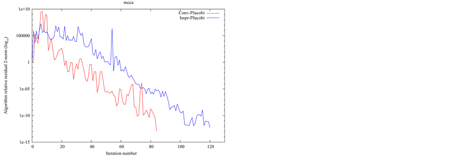
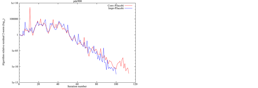
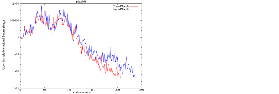
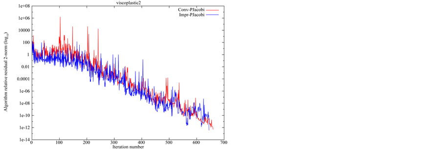
Figure 2.Converging histories of relative residual 2-norm (Jacobi-CGS). Red line: Conventional PCGS, Blue line: Improved PCGS.
Table 3.Numerical results for a veriety of test problems (ILU(0)-CGS).
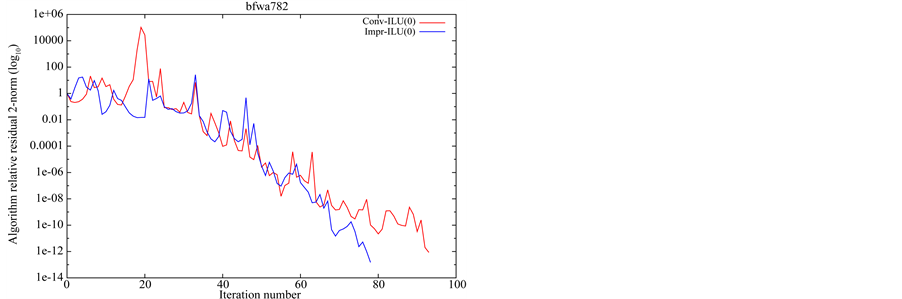
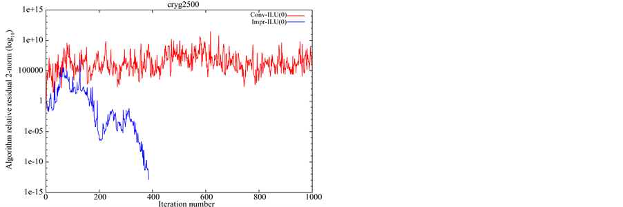
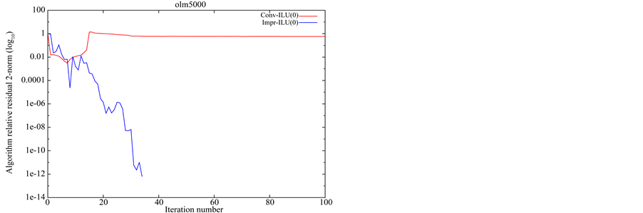
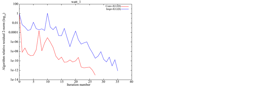
Figure 3.Converging histories of relative residual 2-norm (ILU(0)-CGS). Red line: Conventional PCGS, Blue line: Improved PCGS.
Table 4.Numerical results for a veriety of test problems (SAINV-CGS).
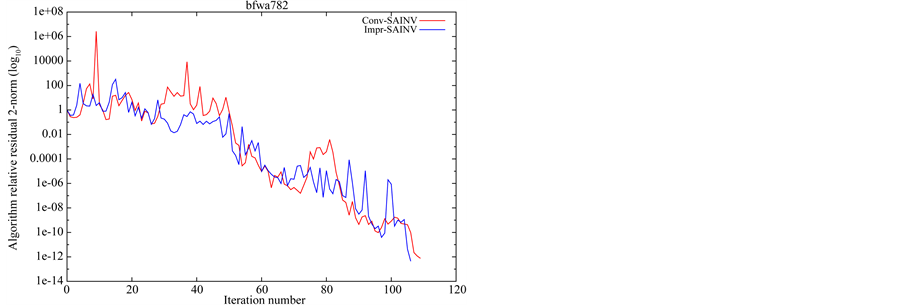
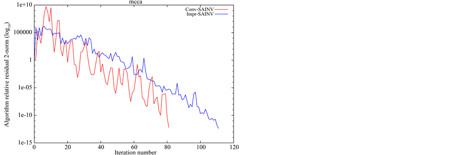
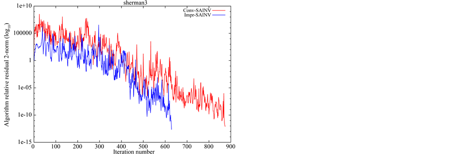
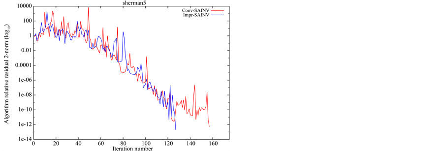
Figure 4. Converging histories of relative residual 2-norm (SAINV-CGS). Red line: Conventional PCGS, Blue line: Improved PCGS.
Table 5. Numerical results for a veriety of test problems (CroutILU-CGS).
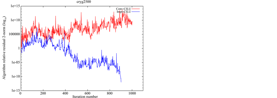
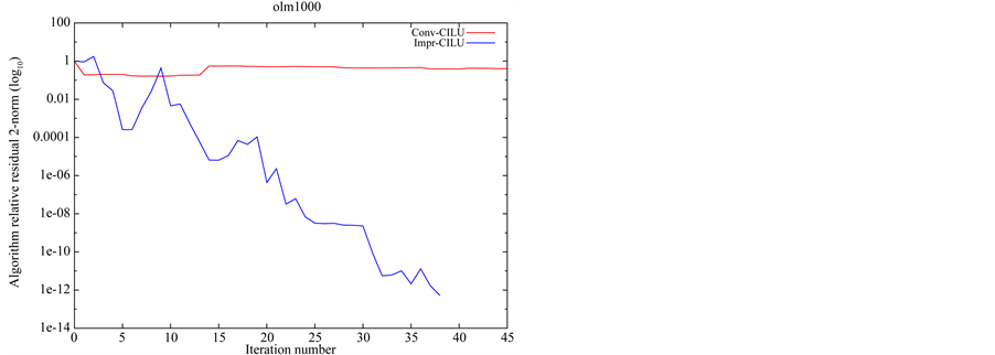
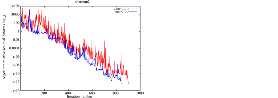
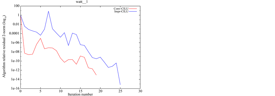
Figure 5. Converging histories of relative residual 2-norm (CroutILU-CGS). Red line: Conventional PCGS, Blue line: Improved PCGS.
Acknowledgements
This work is partially supported by a Grant-in-Aid for Scientific Research (C) No. 25390145 from MEXT, Japan.
Cite this paper
ShojiItoh,MasaakiSugihara, (2015) Formulation of a Preconditioned Algorithm for the Conjugate Gradient Squared Method in Accordance with Its Logical Structure. Applied Mathematics,06,1389-1406. doi: 10.4236/am.2015.68131
References
- 1. Sonneveld, P. (1989) CGS, A Fast Lanczos-Type Solver for Nonsymmetric Linear Systems. SIAM Journal on Scienti fic and Statistical Computing, 10, 36-52.
http://dx.doi.org/10.1137/0910004 - 2. Fletcher, R. (1976) Conjugate Gradient Methods for Indefinite Systems. In: Watson, G., Ed., Numerical Analysis Dundee 1975, Lecture Notes in Mathematics, Vol. 506, Springer-Verlag, Berlin, New York, 73-89.
- 3. Lanczos, C. (1952) Solution of Systems of Linear Equations by Minimized Iterations. Journal of Research of the National Bureau of Standards, 49, 33-53.
http://dx.doi.org/10.6028/jres.049.006 - 4. Van der Vorst, H.A. (1992) Bi-CGSTAB: A Fast and Smoothly Converging Variant of Bi-CG for the Solution of Nonsymmetric Linear Systems. SIAM Journal on Scientific and Statistical Computing, 13, 631-644.
http://dx.doi.org/10.1137/0913035 - 5. Zhang, S.-L. (1997) GPBi-CG: Generalized Product-Type Methods Based on Bi-CG for Solving Nonsymmetric Linear Systems. SIAM Journal on Scientific Computing, 18, 537-551.
http://dx.doi.org/10.1137/s1064827592236313 - 6. Itoh, S. and Sugihara, M. (2010) Systematic Performance Evaluation of Linear Solvers Using Quality Control Techniques. In: Naono, K., Teranishi, K., Cavazos, J. and Suda, R., Eds., Software Automatic Tuning: From Concepts to State-of-the-Art Results, Springer, 135-152.
- 7. Itoh, S. and Sugihara, M. (2013) Preconditioned Algorithm of the CGS Method Focusing on Its Deriving Process. Transactions of the Japan SIAM, 23, 253-286. (in Japanese)
- 8. Hestenes, M.R. and Stiefel, E. (1952) Methods of Conjugate Gradients for Solving Linear Systems. Journal of Research of the National Bureau of Standards, 49, 409-435.
http://dx.doi.org/10.6028/jres.049.044 - 9. Barrett, R., Berry, M., Chan, T.F., Demmel, J., Donato, J., Dongarra, J., et al. (1994) Templates for the Solution of Linear Systems: Building Blocks for Iterative Methods. SIAM.
http://dx.doi.org/10.1137/1.9781611971538 - 10. Van der Vorst, H.A. (2003) Iterative Krylov Methods for Large Linear Systems. Cambridge University Press, Cambridge.
http://dx.doi.org/10.1017/CBO9780511615115 - 11. Meurant, G. (2005) Computer Solution of Large Linear Systems. Elsevier, Amsterdam.
- 12. Davis, T.A. The University of Florida Sparse Matrix Collection.
http://www.cise.ufl.edu/research/sparse/matrices/ - 13. Matrix Market Project.
http://math.nist.gov/MatrixMarket/ - 14. SSI Project, Lis.
http://www.ssisc.org/lis/
NOTES
![]()
1This improved PCGS was proposed in Ref. [7] from a viewpoint of deriving process’s logic, but this manuscript demonstrates some mathematical theorems underlying the deriving process’s logic. Further, numerical results using ILU(0) preconditioner only are shown in Ref. [7] , but the results using a variety of typical preconditioners are shown in this manuscript.

2Of course, [8] discuss the conjugate gradient method for a symmetric system.

8Values of “zero” for ILU(0) indicates the fill-in level, that is, “no fill-in”.
9Because the principal argument presented in this paper concerns the structure of the algorithm for PCGS based on an improved preconditioning transformation procedure, the time required to obtain numerical solutions and the convergence history graphs (Figures 2-5) are provided as a reference. As mentioned before, there is almost no difference between Algorithm 6 and Algorithm 7 as regards the number of operations in the iteration, which would exert a strong influence on the computation time.