Applied Mathematics
Vol.3 No.12A(2012), Article ID:26109,14 pages DOI:10.4236/am.2012.312A300
Measuring Tail Dependence for Aggregate Collateral Losses Using Bivariate Compound Shot-Noise Cox Process
1Department of Applied Finance & Actuarial Studies, Faculty of Business and Economics, Macquarie University, Sydney, Australia
2Benelec Pty Ltd., Sydney, Australia
Email: jiwook.jang@mq.edu.au, paulg@benelec.com.au
Received October 4, 2012; revised November 4, 2012; accepted November 11, 2012
Keywords: Aggregate Collateral Losses; Bivariate Compound Cox Process; Shot Noise Process; Farlie-Gumbel-Morgenstern Copula; Tail Dependence; Joint Fast Fourier Transform
ABSTRACT
In this paper, we introduce tail dependene measures for collateral losses from catastrophic events. To calculate these measures, we use bivariate compound process where a Cox process with shot noise intensity is used to count collateral losses. A homogeneous Poisson process is also examined as its counterpart for the case where the catastrophic loss frequency rate is deterministic. Joint Laplace transform of the distribution of the aggregate collateral losses is derived and joint Fast Fourier transform is used to obtain the joint distributions of aggregate collateral losses. For numerical illustrations, a member of Farlie-Gumbel-Morgenstern copula with exponential margins is used. The figures of the joint distributions of collateral losses, their contours and numerical calculations of risk measures are also provided.
1. Introduction
Over the recent years, numerous papers have looked at the modelling of dependence within an insurance portfolio or between insurance portfolios [1-5]. Also in the field of financial risk management, a range of papers on dependence modelling within credit risk and operational risk can be noticed [6-8]. Besides the construction of specific multivariate models, considerable attraction is given to the use of copulas. In particular, within the theory of Lévy processes, Lévy copulas have proven to be useful [9].
Our paper is very much based on insurance applications where two lines of business are hit by a common external event, hence the word “collateral losses” in the title. These joint losses may, for instance be triggered by events such as flood, windstorm, hail, bushfire, earthquake and terrorism. Particular examples concern collateral losses due to 2011 Great Eastern Japan Earthquake, 2010-2011 Queensland floods, 2009 Victorian Bushfires [10], 2005 Hurricane Katrina [11] and 2001 September 11 attack [12].
For the purpose of this paper, we concentrate on a very specific model and show how, within this model several explicit calculations for relevant risk quantities can be performed. The bivariate model we consider has the following structure:
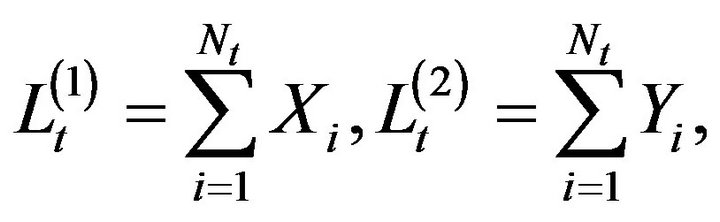 (1)
(1)
where  is the total loss arising from risk type
  and
and  is the number of collateral losses up to time
 . The random variables
  and
and  denote the individual loss amounts. In this model, the dependence between two random variables
  and
and  comes from the common arrival process
 , together with the dependence between the individual losses
  and
and![]() . The latter is modelled using the notion of copula [13]. To be more specific, we assume the loss random variable
. The latter is modelled using the notion of copula [13]. To be more specific, we assume the loss random variable  and
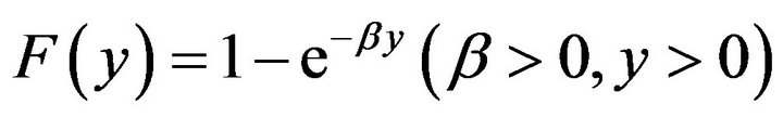
and ![]() are independent identically distributed with continuous distribution function
are independent identically distributed with continuous distribution function  and
and  respectively. The joint distribution of the vector
  is assumed to be of the form
  with a given copula
 . The uniqueness of this two stage construction goes back to Sklar’s Theorem.
Theorem 1.1. (Sklar’s Theorem) Let  be a joint distribution function with margins
  and
and . Then there exists a copula
  such that for all
  in
in 
 (2)
(2)
If the margins are continuous, then C is unique; otherwise C is uniquely determined on , where
  denotes the range of
 . Conversely, if C is a copula and
  and
and  are univariate distribution functions, then the function F defined in (2) is a joint distribution function with margins
  and
and .
.
Proof. See Schweizer and Sklar [14] or Nelsen ([13], p. 18).
To deal with stochastic nature of catastrophic loss arrival in practice, we use a Cox process for . The Cox process provides flexibility by letting the intensity not only depend on time but also allowing it to be a stochastic process. Therefore the Cox process can be viewed as a two step randomisation procedure. A process
  is used to generate another process
  by acting its intensity. That is,
  is a Poisson process conditional on
  which itself is a stochastic process.
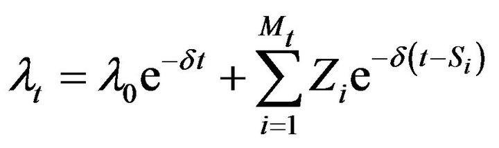
Losses arising from a catastrophe depend on its intensity. One of the processes that can be used to measure the impact of catastrophic events is the shot noise process. Previous works of insurance application using shot noise process and a Cox process with shot noise intensity can be found in [15-19]. Reference [20] also used a Cox process with shot noise intensity to model operational risk. The shot noise process is particularly useful to loss arrival process as it measures the frequency, magnitude and time period needed to determine the effect of catastrophic events. As time passes, the shot noise process decreases as more and more losses are settled. This decrease continues until another event occurs which will result in a positive jump in the shot noise process. Therefore the shot noise process can be used as the parameter of a Cox process to measure the number of catastrophic losses, i.e. we will use it as an intensity function to generate a Cox process. We will adopt the shot noise process used by Cox & Isham [21]:
where:
•  is the initial value of
  that is carried on from catastrophic events incurred previously;
•  is a sequence of independent and identically distributed random variables with distribution function
  and
and  (i.e. magnitude of contribution of catastrophic event
  to intensity);
•  is the sequence representing the event times of a Poisson process
  with constant intensity
 ; and
; and
• ![]() is the rate of exponential decay.
is the rate of exponential decay.
Catastrophic events may take long to materialise so the decay rate may not be exponential. It is assumed to be of this form for a matter of convenience, i.e. closed-form expressions of final results are easily derived. We also make the additional assumption that a Poisson process
 and the sequences
 ,
,  and
and
 are independent of each other.
A Poisson process with loss frequency rate  is also studied for
 , that may be considered when catastrophic loss frequency rate is deterministic.
With the above model specifications, we calculate the following relevant risk measures:
 (3)
(3)
 (4)
(4)
 (5)
(5)
and
 (6)
(6)
Here![]() ,
, ![]() and
and ![]() are the distribution functions of the random variables
are the distribution functions of the random variables ,
,  and
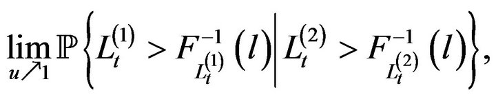
and  respectively. The quantities (3) and (5) are known as asymptotic upper tail dependence measures and the quantities (4) and (6) are conditional tail expectations. The motivation for calculating these quantities that measure extremal dependence in the upper tail of a bivariate distribution is that insurance industry is more concerned with dependence between extreme losses. For a discussion on the coefficient of tail dependence parameters, see McNeil et al. [22].
In order to evaluate above risk measures, we need to obtain the joint distribution of the aggregate collateral losses  and
and . Unfortunately, it is not easy to derive the joint distribution the aggregate collateral losses explicitly. So in Section 2, we derive joint Laplace transform of the distribution of the aggregate collateral losses expressed with a copula function applying the piecewise deterministic Markov processes (PDMPs) theory. For
 , a shot-noise Cox process and a homogeneous Poisson process are used respectively. Section 3 provides the expressions of the moments, covariance and linear correlation between
  and
and  at time
  for both cases. In Section 4, we present the expressions for joint probabilities of the aggregate collateral losses and their densities at
  and
and , which are required to improve the accuracy of the distributions of the aggregate collateral losses inverting joint Fast Fourier transforms. We also provide the figures of the joint distribution of the aggregate collateral losses and their contours. In Section 5, we illustrate the calculations of relevant risk measures (3)-(6) using joint Fast Fourier transforms. For numerical illustrations, an exponential distribution for the jump sizes of catastrophic event, a member of Farlie-Gumbel-Morgenstern copula with exponential margins are used throughout the paper. Section 6 shows the sensitivity analysis on the parameters of a shot-noise Cox process from a Poisson process using the risk measure of (4). Concluding remarks are in Section 7.
2. Joint Laplace Transform of the Distribution of the Aggregate Collateral Losses The piecewise deterministic Markov processes theory developed by Davis [23] is a powerful mathematical tool for examining non-diffusion models. From now on, we present definitions and important properties of  and
and  with the aid of piecewise deterministic Markov processes theory [16,24,25]. This theory is used to derive joint Laplace transform of the distribution of the aggregate collateral losses
  and
and .
.
2.1. Shot-Noise Cox Process
Assuming that the loss arrival process  follows a Cox process with shot noise intensity
 , the generator of the process
  acting on a function
  belonging to its domain is given by
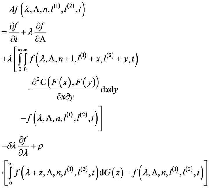
(7)
where . Now let us find a suitable martingale in order to derive joint Laplace transform of the distribution of the aggregate collateral losses
  and
and .
.
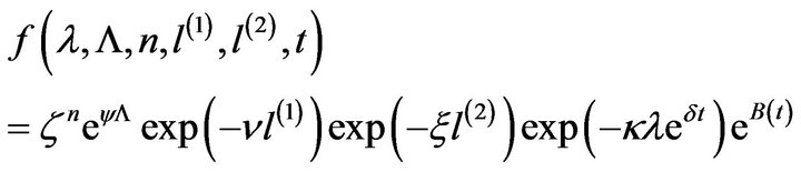
Lemma 2.1. Considering constants
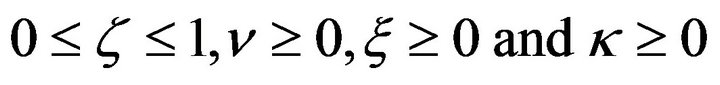 then
then
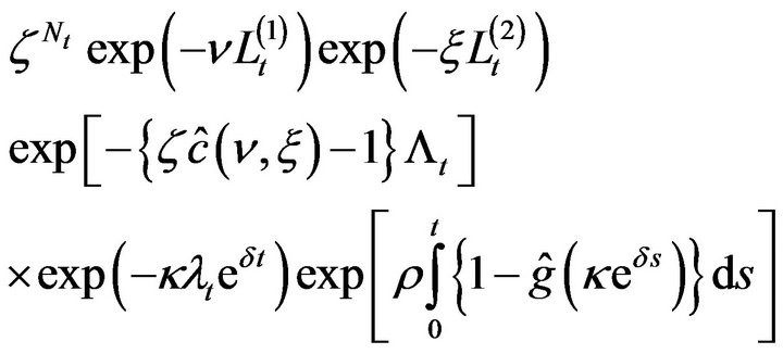 (8)
(8)
is a martingale, where
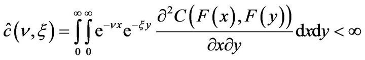 and
and
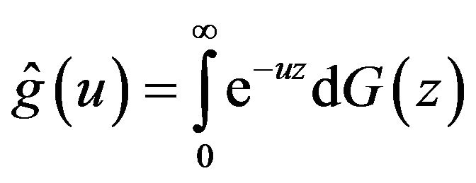 .
.
Proof. From (7),  has to satisfy
 for
for  to be a martingale. Setting
we get the equation
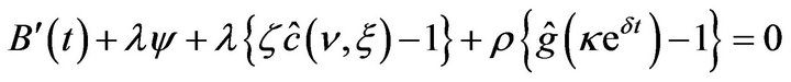 (9)
(9)
and the solution is
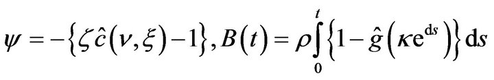 (10)
(10)
by which the result follows.
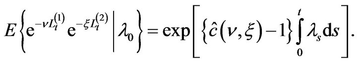
Using the martingale obtained in Lemma 2.1 and setting  and
and  we can easily obtain the general form of joint Laplace transform of the distribution of the aggregate collateral losses
  and
and , i.e.
 (11)
(11)
where the conditional expectation  is based on the probability space
 , and the information set
 with the filtration
 . Without loss of generalitychange the time scale and assume that
  and
and  then it is given by
 (12)
(12)
Throughout the paper, we firstly assume that jump sizes of catastrophic event follow an exponential distribution, i.e. 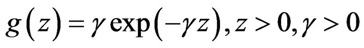 and that
  is stationary. Then using Theorem 2.6 in [16], (12) is given by
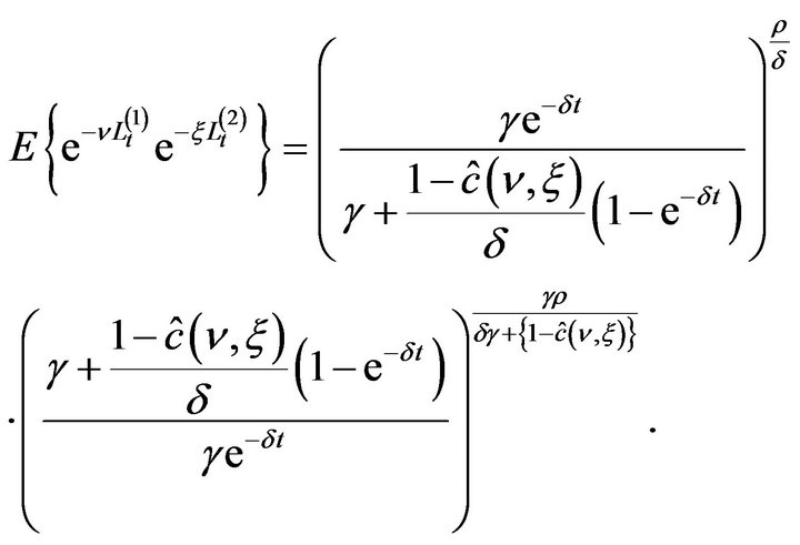 (13)
(13)
Secondly, as a specific example for , we use the Farlie-Gumbel-Morgenstern (FGM) copulas given by
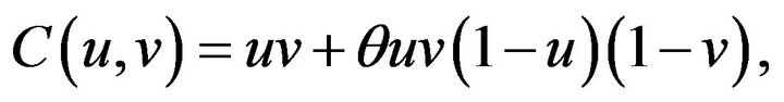 (14)
(14)
where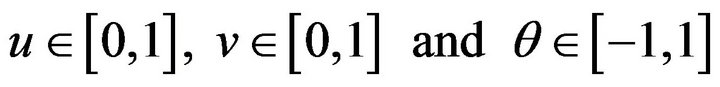 .
.  Lastly, to make this calculation somewhat easier, we assume that
 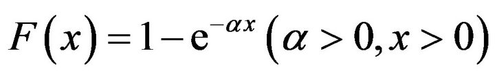 and
and
 . We omit the corresponding expression for the above joint Laplace transform of the distribution of the aggregate collateral losses as it can be easily obtained using the joint distribution function
  driven by (14), i.e.
 (15)
(15)
It will be of interest to examine the joint Laplace transform of the distribution of the aggregate collateral losses  and
and  at time
 , using other copulas and other margins
  and
and . If
. If , which are the magnitude of contribution of catastrophic event to intensity
 , are high, we also need to consider heavy-tailed distributions for jump size of catastrophic event,
 . We also omit the corresponding expressions for the Laplace transform of the distribution of
  which are the Laplace transforms of the distribution of the compound Cox process with shot noise intensity
 , where its jump sizes follow an exponential distribution [16].
If we set  in (15), we have joint Laplace transform of the distribution of the aggregate collateral losses, which is the case that two losses X and Y occur same time from a sharing loss frequency rate
 , but their sizes are independent each other. Due to the dependence of collateral losses of X and Y with sharing loss frequency rate
 , we can see that
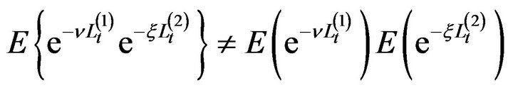 (16)
(16)
even if . If loss
  occurs by arrival process
  with shot noise intensity
  that has three parameters of
 ![]()
 and
and  and loss Y occurs by arrival process
 ![]() with shot noise intensity
with shot noise intensity  that has three parameters of
 and
and  and everything is independent each other, we can have the joint Laplace transform of the distribution of aggregate losses
  and
and  at time t, that is the product of the Laplace transforms of the distribution of
 .
.
2.2. Homogeneous Poisson Process
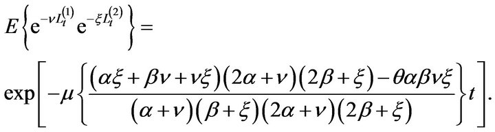
Let us now assume that the loss arrival process  follows a homogeneous Poisson process with loss frequency μ. Setting
  in (12), i.e. considering deterministic loss frequency μ, we can easily obtain that
 (17)
(17)
and using (14) we have
(18)
We omit the corresponding expressions for the Laplace transform of the distribution of  which are the Laplace transforms of the distribution of the compound Poisson process with exponential loss sizes, as they can be easily obtained setting
  and
and  respectively.
Similar to shot-noise Cox process for , due to the dependence of collateral losses of
  and
and ![]() with sharing loss frequency rate
with sharing loss frequency rate  it shows that
 (19)
(19)
even if . If loss
  occurs by arrival process
  with loss frequency
  and loss
 ![]() occurs by arrival process
occurs by arrival process ![]() with loss frequency
with loss frequency  and everything is independent each other, we can also have the joint Laplace transform of the distribution of aggregate losses
  and
and  at time
  that is the product of the Laplace transforms of the distribution of
 .
.
3. Moments, Covariance and Linear Correlation of Aggregate Collateral Losses
In this section, we examine the moments, covariance and linear correlation between  and
and  at time
 . For the loss arrival process
 , we use a Cox process with shot noise intensity
  and a homogeneous Poisson process with loss frequency
 , respectively.
3.1. Shot-Noise Cox Process
Differentiating (12) w.r.t. ![]() and
and  and set
  and
and  we can derive the joint expectation of
  and
and  at time
 , i.e.
 (20)
(20)
Also set  and
and  in (12) and differentiate itw.r.t. v and
  respectively, we can obtain the expectation of
  and
and  at time t, i.e.
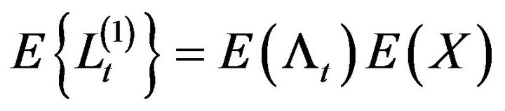 (21)
(21)
and
 (22)
(22)
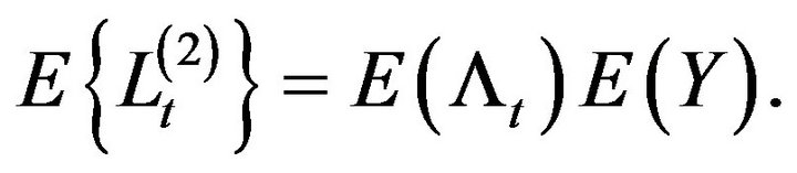
The higher moments of  and
and  at time t can be obtained by differentiating it further, i.e.
 (23)
(23)
and
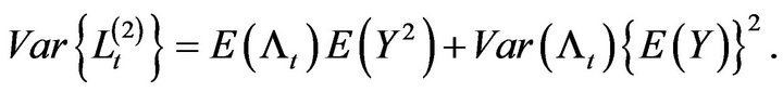 (24)
(24)
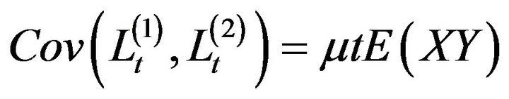
The covariance between  and
and  at time
  is given by
 (25)
(25)
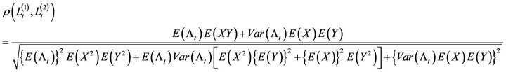
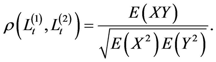
and the linear correlation coefficient between  and
and  at time
  is given by
 (26)
(26)
Let us now illustrate the calculations of the covariance and linear correlation between  and
and  at time
 , where
  follows a shot-noise Cox process.
Example 1
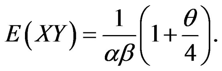
From [17], we have
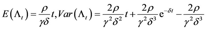
and using (14) we have
The parameter values used to calculate the covariance and linear correlation using (25) and (26) are

Hence from (25) and (26), the calculations of covariance and linear correlation between  and
and  at time
  are shown in Tables 1 and 2 respectively.
3.2. Homogeneous Poisson Process
Similar to a shot-noise Cox process for  differentiating (17) w.r.t.
 ![]() and
and  and set
  and
and  we can easily derive the joint expectation of
  and
and  at time
 , i.e.
 (27)
(27)
We omit the expressions for the expectation and variance of  and
and  at time
  as they can be easily derived similar to a shot-noise Cox process for
 .
.
The covariance between  and
and  at time t is given by
 (28)
(28)
and the linear correlation coefficient between  and
and  at time
  is given by
 (29)
(29)
Let us now illustrate the calculations of the covariance and linear correlation between  and
and  at time
 , where
  follows a Poisson process.
Example 2
The parameter values used to calculate the covariance and linear correlation using (28) and (29) are
From (28) and (29), the calculations of covariance and linear correlation between  and
and  at time
  are shown in Table 3 and Table 4 respectively.
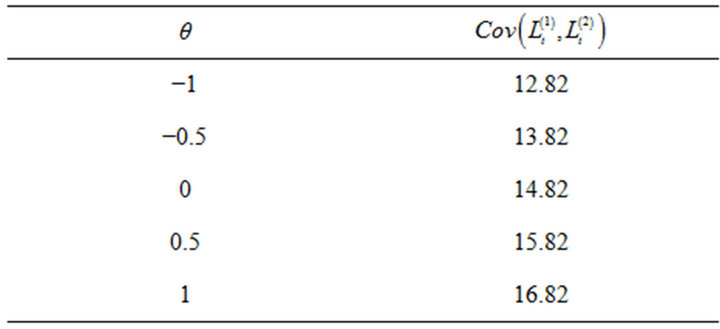
Table 1. Covariance between  and
and .
.
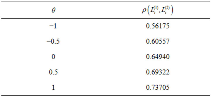
Table 2. Linear correlation between  and
and .
.
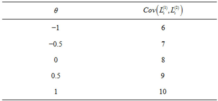
Table 3. Covariance between  and
and .
.
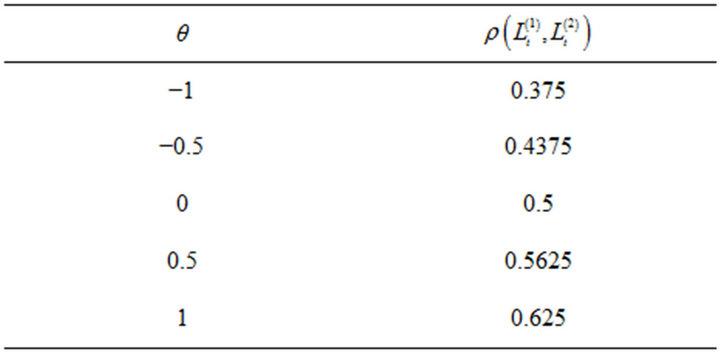
Table 4. Linear correlation between  and
and .
.
3.3. Comparison
The parameter values used in Examples 1-2 provide us with the same means of aggregate collateral losses regardless of the loss arrival process , i.e.
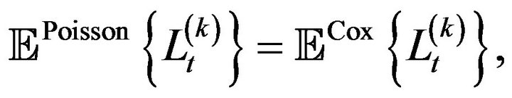
where
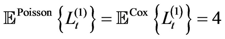 (30)
(30)
and
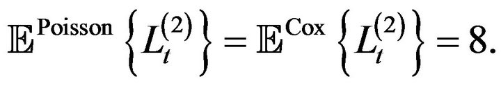 (31)
(31)
However for each  Tables 1 and 3 show that there is an increase in the covariance between
  and
and  by changing
  from a homogenous Poisson process to a shot-noise Cox process. Tables 2 and 4 also show that the linear correlation between
  and
and  increases by changing
  from a homogenous Poisson process to a shot-noise Cox process for each
 . This implies that the marginal distributions of the aggregate collateral loss with respect to a Cox process have heavier tail than their counterparts with respect to a Poisson process, i.e.
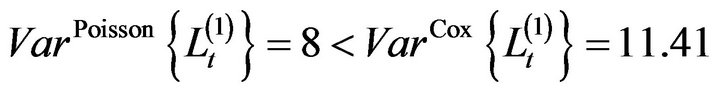 (32)
(32)
and
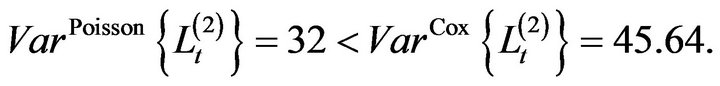 (33)
(33)
It will also become apparent by the joint distributions of aggregate collateral losses and their contours in Section 4 and numerical risk measure values in Examples 3- 6.
4. Joint Distribution of the Aggregate Collateral Losses via Bivariate Fast Fourier Transform
In order to calculate the risk measures of (3)-(6), we invert bivariate Fast Fourier transforms from joint Laplace transforms of the vector  obtained in Section 2. For details on how to use bivariate Fast Fourier transform, we refer to [26-28]. Before we show the calculations of risk measures in Section 5, we present the expressions for the joint probabilities of the aggregate collateral losses and their densities at
  and
and . These are required to improve the accuracy of the joint distributions of the aggregate collateral losses inverting bivariate Fast Fourier transforms.
4.1. Shot-Noise Cox Process
If we let ![]() and
and  in (13), we have the expression for the joint probability of aggregate collateral losses at
  and
and , i.e.
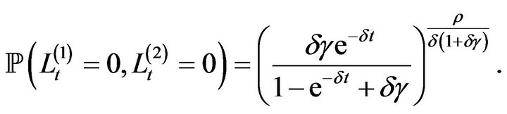 (34)
(34)
Regardless of loss size distributions, we have the same joint probability of aggregate collateral losses at  and
and  when the loss arrival process
  follows a Cox process with shot noise intensity
 . If we set
the expression for the joint density of aggregate collateral losses at  and
and  is given by
 (35)
(35)
Based on (35), we can easily obtain its expression for exponential loss sizes using (14), i.e.
 (36)
(36)
Figures 1-4 are the joint distributions of aggregate collateral losses and their contours at each value of  with respect to a shot-noise Cox process for
 .
.
Figure 2 (or Figure 1) shows that joint probabilities of aggregate collateral losses are mainly located between the bottom left corner and the top right corner when , which means loss
  and
and ![]() move in the same direction. On the other hand, compared to when
move in the same direction. On the other hand, compared to when , Figure 4 (or Figure 3) shows that joint probabilities of aggregate collateral losses at the bottom left corner and the top right corner moves to its diagonal left and right, respectively when
  which means loss
  and
and ![]() move in the opposite direction.
move in the opposite direction.
4.2. Homogeneous Poisson Process
If we let ![]() and
and  in (18), we have the expression for the joint probability of aggregate collateral losses at
  and
and , i.e.
 (37)
(37)
Regardless of loss size distributions, we have the same joint probability of aggregate collateral losses at  and
and  when the loss arrival process
  follows a homogeneous Poisson process with loss frequency
 . If we set
the expression for the joint density of aggregate collateral losses at  and
and  is given by
 (38)
(38)
Based on (38), we can easily obtain its expression for exponential loss sizes using (14), i.e.
 (39)
(39)
The figures of the joint distributions of aggregate collateral losses and their contours at each value of  with respect to a Poisson process for
  are omitted, for which see the early version of this paper in http://ssrn.com/author=383758.
5. Calculating Risk Measures for Collateral Losses Now using the parameter values in Examples 1-2 and Matlab, let us illustrate the calculations of the risk measures of (3)-(6) with respect to a shot-noise Cox process and a Poisson process. They are shown in Tables 5-18.
To reduce the error of used algorithm for inverting bivariate Fast Fourier transforms using Matlab, the following methods have been used:
• The sampling points have been taken as many as possible, i.e. we have used 8192 × 4096 points in the calculation, which was the maximum points we could sampled in 32-bit Matlab.
• If the sampling interval gap is too small, there would be a large amount of truncation error. Also if the sampling interval is too big, there would be a large amount of sampling error. Hence we have chosen carefully the right sampling interval, so that the total errors caused by inverting bivariate Fast Fourier transforms could be negligible.
• For the figures in this paper, we have used the 2D
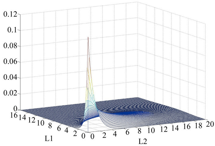
Figure 1. The joint distribution of collateral losses with θ = 1.
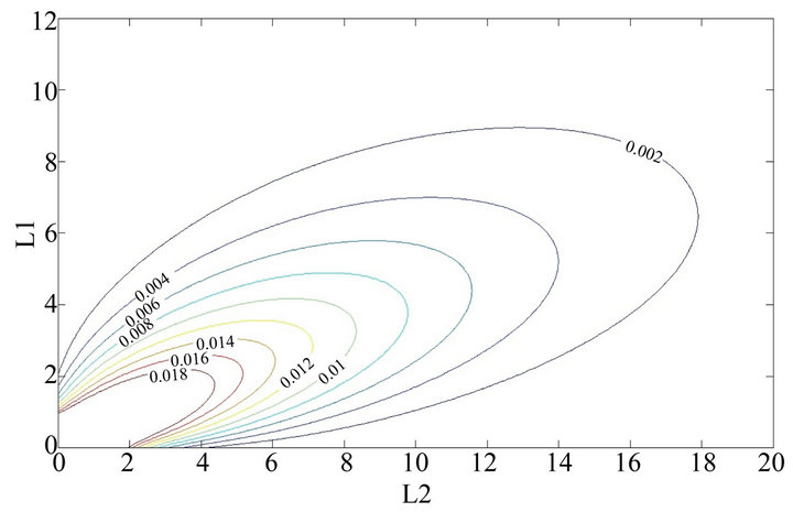
Figure 2. The contour of the joint distribution of collateral losses with θ = 1.
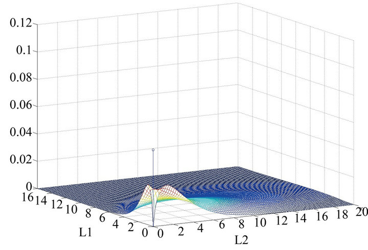
Figure 3. The joint distribution of collateral losses with θ = −1.
low-pass/moving-average filter to filter the jitter noise out. Then we have used the linear interpolation to smooth the borders of the data. The pattern matrix used for this filter was
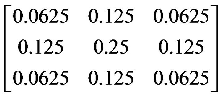 .
.
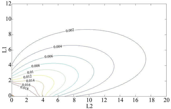
Figure 4. The contour of the joint distribution of collateral losses with θ = −1.
Example 3
Using the different  at
at  and
and , the calculations of the risk measure of (3) are shown in Tables 5-8.
Tables 5-8 show that each quantile values are higher with respect to a shot-noise Cox process than their counterparts. They also show that the risk measures of (3) with respect to a shot-noise Cox process are higher than their counterparts. These justify that the marginal/joint distributions of the aggregate collateral losses with respect to a shot-noise Cox process have heavier tail than their counterparts with respect to a Poisson process.
Example 4
Secondly, based on the  at 95% and 99% in Example 3, the calculations of the risk measure (4), i.e.
 are shown in Tables 9 and 10.
Tables 9 and 10 show that the risk measures of (4) with respect to a shot-noise Cox process are higher than their counterparts regardless of the critical values. Regardless of the loss arrival process , the risk measures of (4) are getting bigger as the critical value goes to 99%. They also show that the differences between the values in Table 9 and their counterparts in Table 10 are getting higher as the critical value goes to 99%.
Example 5
Showing the calculations of the  quantiles of the sum,
  , i.e.
  in
in
 and the joint probability between
  and
and  i.e.
i.e.  for each cases in Tables 11-14, the calculations of the risk measure (5) are shown in Tables 15 and 16.
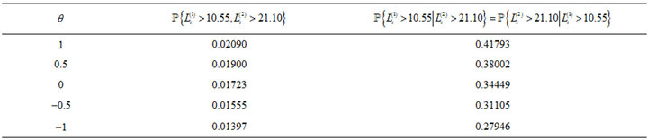
Table 5. A shot-noise Cox process, where![]() .
.
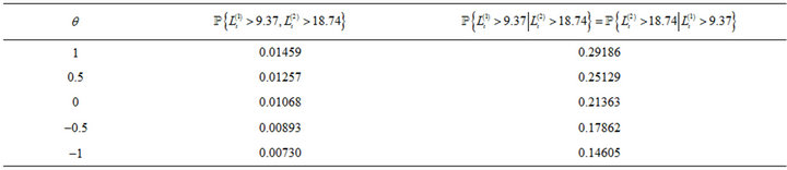
Table 6. A Poisson process, where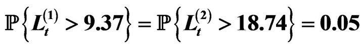 .
.
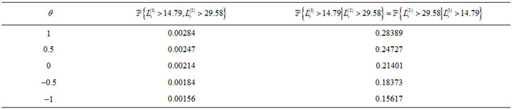
Table 7. A shot-noise Cox process, where![]() .
.
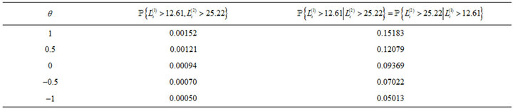
Table 8. A Poisson process, where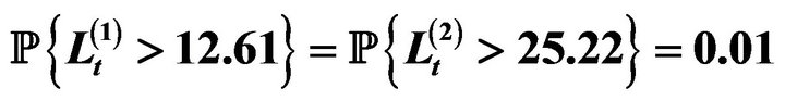 .
.
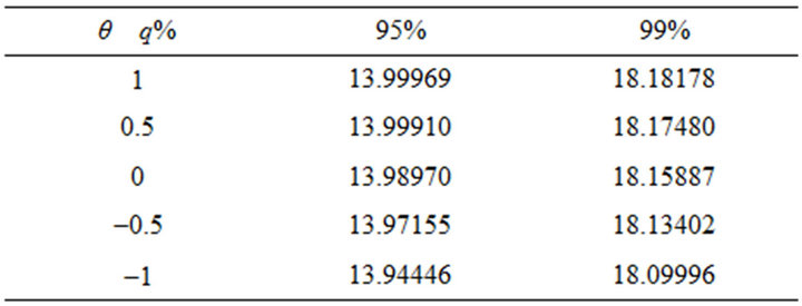
Table 9. A shot-noise Cox process.
Table 10. A Poisson process.
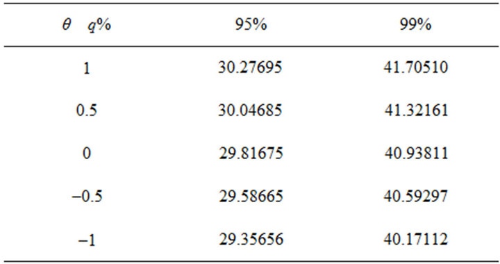
Table 11.  quantiles of the sum,
  for a shotnoise Cox process.
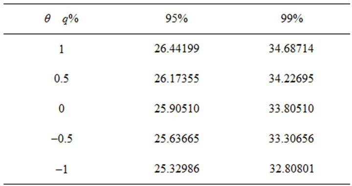
Table 12.  quantiles of the sum,
  for a poisson process
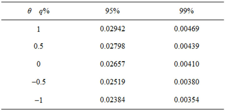
Table 13. 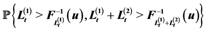 for a shot-noise Cox process.
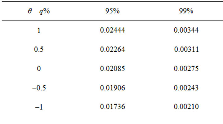
Table 14.  for a Poisson process.
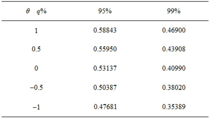
Table 15. 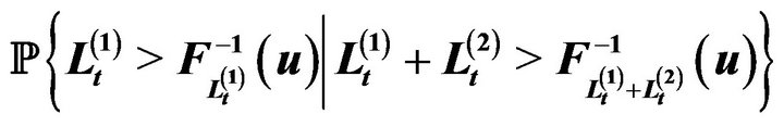 for a shot-noise Cox process.
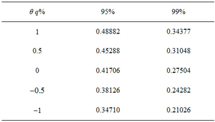
Table 16. 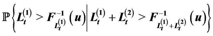 for a Poisson process.
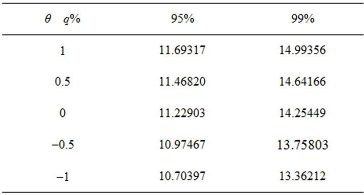
Table 17. A shot-noise Cox process.
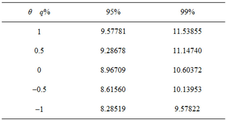
Table 18. A Poisson process.
Tables 11 and 12 show that the  quantiles of the sum,
  with respect to a shot-noise Cox process are higher than their counterparts regardless of the critical values. Regardless of the loss arrival process
 , they are getting bigger as the critical value goes to
 . They also show that the differences between the values in Table 11 and their counterparts in Table 12 are getting higher as the critical value goes to 99.9%.
Tables 13 and 14 show that the joint probability between  and
and  with respect to a shot-noise Cox process are higher than their counterparts regardless of the critical values. Regardless of the loss arrival process
 , they are getting smaller as the critical value goes to 99.9%. They also show that the differences between the values in Table 13 and their counterparts in Table 14 are getting lower as the critical value goes to 99.9%.
Tables 15 and 16 show that the risk measures of (5) with respect to a shot-noise Cox process are higher than their counterparts regardless of the critical values. Regardless of the loss arrival process , the risk measures of (5) are getting smaller as the critical value goes to 99.9%.
Example 6
Lastly, based on the quantile values and the joint probabilities in Example 5, the calculations of the risk measure (6), i.e.  are shown in Tables 17 and 18.
Tables 17 and 18 show that the risk measures of (6) with respect to a shot-noise Cox process are higher than their counterparts regardless of the quantile values. Regardless of the loss arrival process , the risk measures of (6) are getting bigger as the critical value goes to
 . They also show that the differences between the values in Table 17 and their counterparts in Table 18 are getting higher as the critical value goes to 99.9%.
With respect to the FGM copula correlation parameter,  , the risk measures of (3)-(6) are increasing (decreasing) as it changes to
  regardless of the loss arrival process
 . It will be interesting to find these risk measure values using other copulas with different marginal distributions.
6. Sensitivity Analysis In this section, we examine the effect on the risk measure of (4), i.e.
caused by changes in the values of the parameters of a shot-noise Cox process from a Poisson process. To do so, we double the means of aggregate collateral losses, (30) and (31) with  for a Poisson case and with
 and
and  respectively for shotnoise Cox case, i.e.
and
where other parameter values are the same as in Examples 1-2.
Figures 5-6 are the joint distribution of aggregate collateral losses and its contour at  with respect to a Poisson process for
 . Figures 7-12 are the joint distributions of aggregate collateral losses and their con-
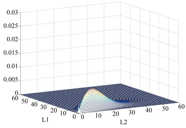
Figure 5. The joint distribution of collateral losses with θ = 1 for a Poisson process.
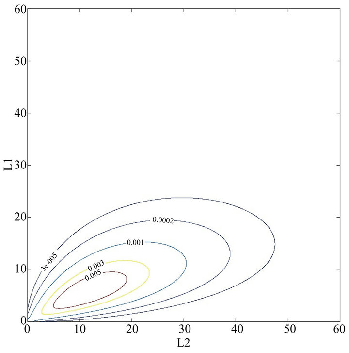
Figure 6. The contour of the joint distribution of collateral losses with θ = 1 for a Poisson process.
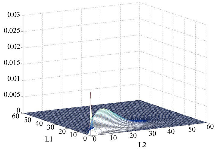
Figure 7. The joint distribution of collateral losses with θ = 1 and ρ = 4.
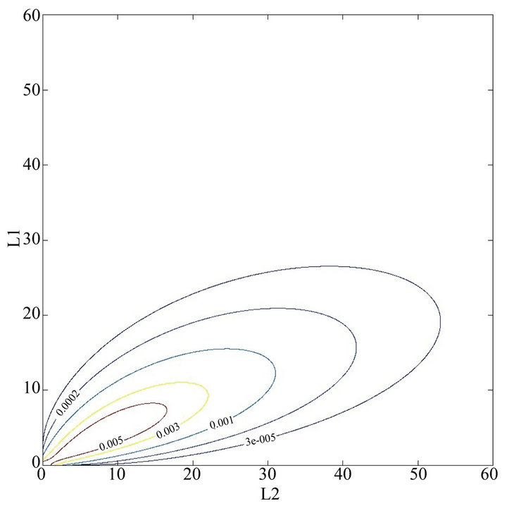
Figure 8. The contour of the joint distribution of collateral losses with θ = 1 and ρ = 4.
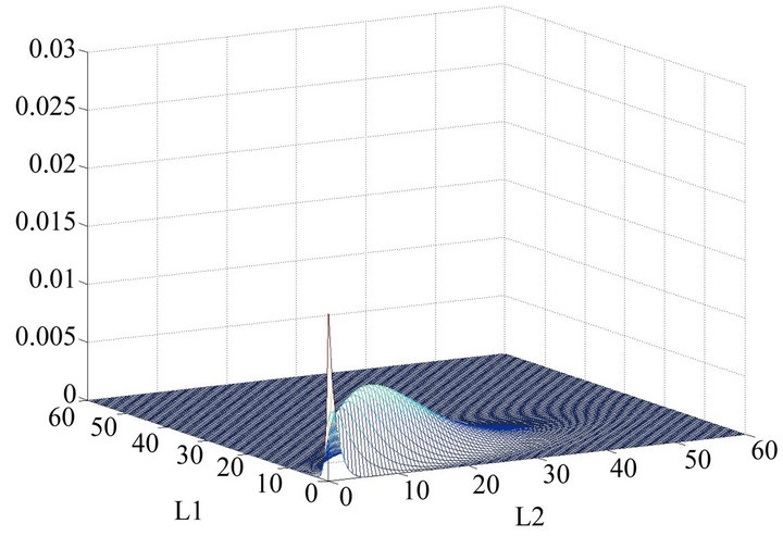
Figure 9. The joint distribution of collateral losses with θ = 1 and δ = 0.25.
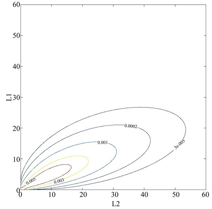
Figure 10. The contour of the joint distribution of collateral losses with θ = 1 and δ = 0.25.
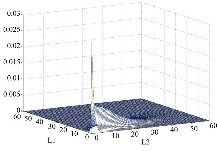
Figure 11. The joint distribution of collateral losses with θ = 1 and γ = 0.5.
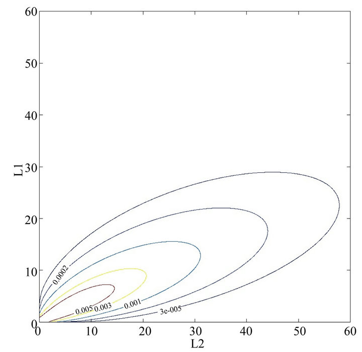
Figure 12. The contour of the joint distribution of collateral losses with θ = 1 and γ = 0.5.
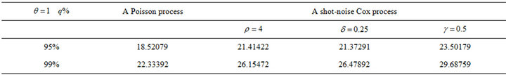
Table 19.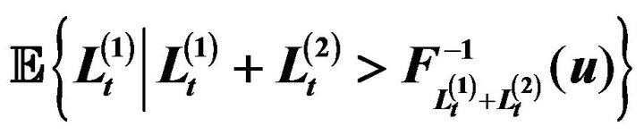 .
.
tours at  with respect to a shot-noise Cox process for
 .
.
Figures 7-12 (shot-noise Cox cases) show how different joint probabilities of aggregate collateral losses are from Figures 5-6 (a Poisson case) by changes in the value of , respectively. Even though they have the same mean, the joint probabilities of aggregate collateral losses for shot-noise Cox cases are located more between the bottom left corner and the top right corner when
  than its counterpart. Shot-noise Cox cases display that they have heavier tail than their counterparts, which are shown in Table 19 in terms of the risk measure of (4). Compared to the effect on the risk measure of (4) by changes in the value of
 , respectively from a Poisson case, Table 19 shows that
 , which is the parameter in exponential jump size distribution of catastrophic event, is the most sensitive parameter in terms of changes in the value the risk measure of (4).
7. Conclusions
We have used bivariate compound process to model aggregate collateral losses arising from catastrophic events such as flood, storm, hail, bushfire and earthquake. For the number of collateral losses, a Cox process was used to accommodate the stochastic nature of their frequency rate in practice. The shot noise process was used as the intensity of a Cox process as the number of collateral losses arising from catastrophic events depends on the frequency and magnitude of the primary events and the time period needed to determine the effect of these events. We also examined a Poisson process for the number of collateral losses as its counterpart. With the common collateral loss arrival process in the bivariate model, the dependence between the individual losses arising from different risk type has been modelled using the notion of copula where for numerical illustrations, a member of Farlie-Gumbel-Morgenstern copula with exponential margins was used.
As it was difficult to derive the joint distributions the aggregate collateral losses, we derived their Laplace transforms and inverted their Fast Fourier transforms numerically to calculate introduced relevant risk measures. These measures can be used to calculate tail dependences between collateral losses or to calculate insurance premiums. We have presented the expressions for joint probabilities of the aggregate collateral losses and their densities at  and
and , which were used to improve the accuracy of joint distributions of the aggregate collateral losses inverting the Fast Fourier transforms. We have compared the simulated risk measure values obtained using a compound Poisson and a compound shot-noise Cox model, respectively. The sensitivity analysis on the parameters of a shot-noise Cox process from a Poisson process also provided using the risk measure of (4).
Other counting processes and other copulas with different margins can be considered in the proposed bivariate model, that we leave for further research. We hope that what we have presented in this paper provides practitioners with feasible models to quantify collateral losses that would occur more often due to global warming, climate change and terrorism.
REFERENCES
- N. Bäuerle and A. Müller, “Modeling and Comparing Dependencies in Multivariate Risk Portfolios,” ASTIN Bulletin, Vol. 28, No. 1, 1998, pp. 59-76. doi:10.2143/AST.28.1.519079
- H. Cossette, P. Gaillardetz, E. Marceau and J. Rioux, “On Two Dependent Individual Risk Models,” Insurance: Mathematics and Economics, Vol. 30, No. 2, 2002, pp. 153-166. doi:10.1016/S0167-6687(02)00094-X
- C. Genest, E. Marceau and M. Mesfioui, “Compound Poisson Approximations for Individual Models with Dependent Risks,” Insurance: Mathematics and Economics, Vol. 32, No. 1, 2003, pp. 73-91. doi:10.1016/S0167-6687(02)00205-6
- N. Bäuerle and R. Grübel, “Multivariate Counting Processes: Copulas and Beyond,” ASTIN Bulletin, Vol. 35, No. 2, 2005, pp. 379-408. doi:10.2143/AST.35.2.2003459
- M. L. Centeno, “Dependent Risks and Excess of Loss Reinsurance,” Insurance: Mathematics and Economics, Vol. 37, No. 2, 2005, pp. 229-238. doi:10.1016/j.insmatheco.2004.12.001
- F. Lindskog and A. J. McNeil, “Common Poisson Shock Models: Applications to Insurance and Credit Risk Modelling,” ASTIN Bulletin, Vol. 33, No. 2, 2003, pp. 209- 238. doi:10.2143/AST.33.2.503691
- D. Pfeifer and J. Nešlehová, “Modeling and Generating Dependent Risk Processes for IRM and DFA,” ASTIN Bulletin, Vol. 34, No. 2, 2004, pp. 333-360. doi:10.2143/AST.34.2.505147
- V. Chavez-Demoulin, P. Embrechts and J. Nešlehová, “Quantitative Models for Operational Risk: Extremes, Dependence and Aggregation,” Journal of Banking and Finance, Vol. 30, No. 10, 2006, pp. 2635-2658. doi:10.1016/j.jbankfin.2005.11.008
- R. Cont and P. Tankov, “Financial Modelling with Jump Processes,” Champan & Hall, Boca Raton, 2004.
- Victorian Bushfires Royal Commission, “Final ReportSummary, Parliament of Victoria,” Parliament of Victoria, Melbourne, 2010.
- M. L. Burton and M. J. Hicks, “Hurricane Katrina: Preliminary Estimates of Commercial and Public Sector Damages,” Marshall University, Huntington, 2005.
- G. Makinen, “The Economic Effects of 9/11: A Retrospective Assessment,” Congressional Research Service, Washington DC, 2002.
- R. B. Nelsen, “An Introduction to Copulas,” SpringerVerlag, New York, 1999.
- B. Schweizer and A. Sklar, “Probabilistic Metric Spaces,” Elsevier, New York, 1983.
- C. Klüppelberg and T. Mikosch, “Explosive Poisson Shot Noise Processes with Applications to Risk Reserves,” Bernoulli, Vol. 1, No. 1-2, 1995, pp. 125-147. doi:10.2307/3318683
- A. Dassios and J. Jang, “Pricing of Catastrophe Reinsurance & Derivatives Using the Cox Process with Shot Noise Intensity,” Finance & Stochastics, Vol. 7, No. 1, 2003, pp. 73-95. doi:10.1007/s007800200079
- A. Dassios and J. Jang, “Kalman-Bucy Filtering for Linear System Driven by the Cox Process with Shot Noise Intensity and Its Application to the Pricing of Reinsurance Contracts,” Journal of Applied Probability, Vol. 42, No. 1, 2005, pp. 93-107. doi:10.1239/jap/1110381373
- A. Dassios and J. Jang, “The Distribution of the Interval between Events of a Cox Process with Shot Noise Intensity,” Journal of Applied Mathematics and Stochastic Analysis, Vol. 2008, 2008, Article ID: 367170. doi:10.1155/2008/367170
- J. Jang and Y. Krvavych, “Arbitrage-Free Premium Calculation for Extreme Losses Using the Shot Noise Process and the Esscher Transform,” Insurance: Mathematics and Economics, Vol. 35, No. 1, 2004, pp. 97-111. doi:10.1016/j.insmatheco.2004.05.002
- J. Jang and G. Fu, “Transform Approach for Operational Risk Management: VaR and TCE,” Journal of Operational Risk, Vol. 3, No. 2, 2008, pp. 45-61.
- D. R. Cox and V. Isham, “Point Processes,” Chapman & Hall, London, 1980.
- A. McNeil, R. Frey and P. Embrechts, “Quantitative Risk Management: Concepts, Techniques and Tools,” Princeton University Press, Princeton, 2005.
- M. H. A. Davis, “Piecewise Deterministic Markov Processes: A General Class of Non Diffusion Stochastic Models,” Journal of the Royal Statistical Society Series B, Vol. 46, No. 3, 1984, pp. 353-388.
- A. Dassios and P. Embrechts, “Martingales and Insurance Risk,” Communications in Statistics. Stochastic Models, Vol. 5, No. 2, 1989, pp. 181-217. doi:10.1080/15326348908807105
- T. Rolski H. Schmidli, V. Schmidt and J. L. Teugels, “Stochastic Processes for Insurance and Finance,” John Wiley & Sons, Hoboken, 1998.
- K. R. Castleman, “Digital Image Processing,” Prentice Hall, Englewood Cliffs, 1996.
- R. C. Gonzalez and R. E. Woods, “Digital Image Processing,” 2nd Edition, Prentice Hall, Upper Saddle River, 2002.
- R. C. Gonzalez, R. E. Woods and S. L. Eddins, “Digital Image Processing Using MATLAB,” Prentice Hall, Upper Saddle River, 2004.