Applied Mathematics
Vol. 3 No. 6 (2012) , Article ID: 20360 , 10 pages DOI:10.4236/am.2012.36099
Hopf Bifurcations in a Predator-Prey System of Population Allelopathy with Discrete Delay
Department of Mathematics, Yunnan Normal University, Kunming, China
Email: wxhwj2005@163.com, liuwang.2011@yahoo.cn
Received December 29, 2011; revised May 2, 2012; accepted May 9, 2012
Keywords: Lotka-Volterra Predator-Prey System; Discrete Delay; Allelopathy; Stability; Hopf Bifurcation; Periodic Solution
ABSTRACT
A delayed Lotka-Volterra two-species predator-prey system of population allelopathy with discrete delay is considered. By linearizing the system at the positive equilibrium and analyzing the associated characteristic equation, the asymptotic stability of the positive equilibrium is investigated and Hopf bifurcations are demonstrated. Furthermore, the direction of Hopf bifurcation and the stability of the bifurcating periodic solutions are determined by the normal form theory and the center manifold theorem for functional differential equations (FDEs). Finally, some numerical simulations are carried out for illustrating the theoretical results.
1. Introduction
In recent years, the Lotka-Volterra predator-prey models modeled by ordinary differential equations (ODEs) have been proposed and studied extensively since the pioneering theoretical works by Lotka [1] and Volterra [2]. With the modification of Brelot [3], the model has the form
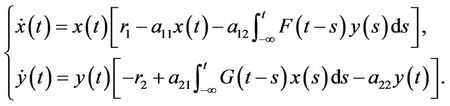 (1)
(1)
where ,
,  ,
,  and
and 
 . Models such as (1) with various delay kernels and delayed Intraspecific competetions have been investigated extensively by many researchers; see reference [4-12] for detail. For example, when F(s) = δ(s − τ) (τ ≥ 0), then system (1) is reduced to the following Lotka-Volterra two-species predator-prey system with a discrete delay and a distributed delay:
 (2)
(2)
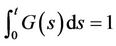
The delay kernel function G(s) may take the so-called “weak” generic kernel function G(s) =  (α > 0) and “strong” generic kernel function G(s) =
  (α > 0), where the “weak” generic kernel implies that the importance of events in the past simply decreases exponentially the further one looks into the past while the “strong” generic kernel implies that a particular time in the past is more iportant than any other [13]. When G(s) takes the “weak” generic kernel function and the “strong” generic kernel function G(s) =
  (α > 0), properties of the stability of the positive equilibrium of system (2) and Hopf bifurcations of nonconstant periodic solutions have been investigated respectively by using the normal form theory and the center manifold reduction for FDEs [14,15]. See [5,16] for details.
When F(s) = δ(s − τ) (τ ≥ 0) and G(s) = δ(s − η) (η ≥ 0) where δ denotes Dirac delta function. Then system (1) is transformed into the following form with two different discrete delays
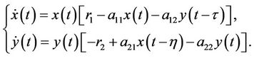 (3)
(3)
He [17] and Lu andWang [18] investigated the stability of the positive equilibrium of the system, and they found that the positive equilibrium is globally asymptotically stable for any values of delays τ and η when the coefficients of the system satisfy the condition 
 > 0 when η > 0, and consider η or the sum of two delays τ and η as the bifurcation parameter, one can see [6-8] for details. Yan and Zhang [9] studied the effect of delay on the dynamics of system (3) when τ = η. Furthermore, for the study of system (3) with delayed intra-specific competitions, one can refer to [10,11].
For Latka-Volterra two species competition model, an important observation made by many works is that increased population of one species might affect the growth of another species by the production of allelopathic toxins or stimulators, thus influencing seasonal succession [19]. For instance, Maynard Smith [20] incorporated the effect of toxic substances in a two species Lotka-Volterra competitive system by considering that each species produce a substance toxic to the other but only when the other is present. Then the Lotka-Volterra competitive system was modified into the form:
 (4)
(4)
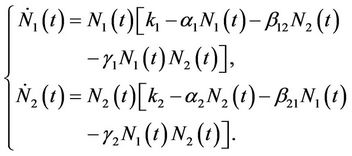
Chattopadyay [21] studied the stability properties of the above system, although the study contains the flaw of ignoring an important delay factor in the system. [22] suggested “In reality, a species needs sometime for maturity to produce a substance which will be toxic (or stimulatory) to the other and hence a delay term in the system arises”. Mukhopadhyay, Chattpadhyay and Tapaswi [22] introduced a delay in system (4), which leads the following form
 (5)
(5)
When γ1 > 0, γ2 > 0, the model system (5) represents an allelopathic inhibitory system, each species producing a substance toxic to the other; when γ1 < 0, γ2 < 0, (5) repr esents an allelopathic stimulatory system, each species producing a substance stimulatory to the growth of the other species.
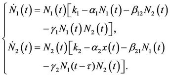
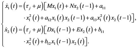
Similar phenomenon also exist in predator-prey model. Rice [19] has suggested that “all meaningful, functional ecological models will eventually have to include a category on allelopathic and other allelochemic effects”. To our knowledge, such viewpoint haven’t been investigated in predator-prey model so far. On the other hand, some species in the real nature world may produce substances which are toxic or stimulatory to the others while they themselves do not experience any reciprocal effects during the process of predation. For example, some species of poisonous snake release toxic substance to control prey. The production of toxic substance by the predator species will not be instantaneous, but mediated by some time lag, see [7,19-22]. From this viewpoint and combining the factors appeared above of different type of time delay and allelopathic effect in predator-prey model, we have modified the model of (3). Therefore, by considering that one species produced a substance toxic to the other during the process of predation, but only when the other is present. Then the system (3) can be written as
 (6)
(6)
where ,
,  ,
,  (i, j = 1, 2),
 . We have investigated the bifurcation behavior on time delay of this modified dynamical system (6). It has also been observed that time delay can drive the competitive system to sustained oscillations, as shown by Hopf bifurcation analysis and limit cycle stability. Hence interaction between the time delay effect produced by delayed toxin can regulate the densities of different competing species in the aquatic ecosystem, thus influencing seasonal successsion, blooms and pulses. To the best of our knowledge no such attempts have been taken to include interaction between the time delay effect produced by delayed toxin in a predator-prey system. Therefore, this research might behelpful to the study of predator-prey model and related problem in biological system.
This paper is organized as follows. In Section 2, by linearizing the resulting two-dimensional system at the positive equilibrium and analyzing the associated characteristic equation, it is found that under suitable conditions on the parameters the positive equilibrium is asymptotically stable when the delay is less than a certain critical value and unstable when the delay is greater than this critical value. Meanwhile, according to the Hopf bifurcation theorem for FDEs, we find that the system can also undergo a Hopf bifurcation of nonconstant periodic solution at the positive equilibrium when the delay crosses through a sequence of critical values. In Section 3, to determine the direction of the Hopf bifurcations and the stability of bifurcated periodic solutions occurring through Hopf bifurcations, an explicit algorithm is given by applying the normal form theory and the center manifold reduction for FDEs developed by Hassard, Kazarinoff and Wan [23]. To verify our theoretical predictions, some numerical simulations are also included in Section 4.
2. Stability of Equilibria and Existence of Hopf Bifurcations
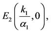
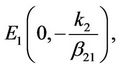
The state of equilibria of the system (6) for τ = 0 are as follows:


where
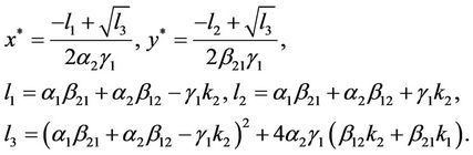
 is a unique positive equilibrium when the condition (H1)
  holds. Throughout this section, we always assume that the condition H(1) holds.
Clearly, the characteristic equation of the linearized system of system (6) at the equilibrium  is
is

which has two real roots,  ,
, . Therefore, the equilibrium
  is unstable and is a saddle point of system (6). The linearized system of system (6) at the equilibrium
  is
is
which has two real roots,  ,
, . Therefore, the equilibrium
 , is an unstable node of system (6). The characteristic equation at the equilibrium
  resulting from the linear system (6) has the form
 . Under the condition (H1), Equation (7) has a negative real root
  and a positive real root
 . Therefore, the equilibrium
  is unstable and is also a saddle point of system (6) when the condition (H1) is satisfied.
In what follows, we investigate the stability of the positive equilibrium  of system (6).
Underthe assumption (H1), let ,
,  . Then system (6) is equivalent to the following two dimensional system:
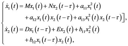 (8)
(8)
where
and the positive equilibrium  of system (6) is transformed into the zero equilibrium (0, 0) of system (8). It is easy to see that the characteristic equation of the linearized system of system (8) at the zero equilibrium (0, 0) is
 (9)
(9)
where b0 = −ND, a0 = ME, a1 = −(M + E).
It is well known that the stability of the zero equilibrium (0, 0) of system (8) is determined by the real parts of the roots of Equation (9). If all roots of Equation (9) locate the left-half complex plane, then the zero equilibrium (0, 0) of system (8) is asymptotically stable. If Equation (9) has a root with positive real part, then the zero solution is unstable. Therefore, to study the stability of the zero equilibrium (0, 0) of system (8), an important problem is to investigate the distribution of roots in the complex plane of the characteristic Equation (9).
For Equation (9), according to the Routh-Hurwitz criterion, we have the following result.
Lemma 2.1. The two roots of Equation (9) with τ = 0 have always negative real parts, the zero equilibrium (0,0) of system (8) with τ = 0 is asymptotically stable.
Next, we consider the effects of a positive delay τ on the stability of the zero equilibrium (0, 0) of system (8). Since the roots of the characteristic Equation (9) depend continuously on τ, a change of τ must lead to a change of the roots of Equation (9). If there is a critical value of τ such that a certain root of (9) has zero real part, then at this critical value the stability of the zero equilibrium (0, 0) of system (8) will switch, and under certain conditions a family of small amplitude periodic solutions can bifurcate from the zero equilibrium (0, 0); that is, a Hopf bifurcation occurs at the zero equilibrium (0, 0).
Now, we look for the conditions under which the characteristic Equation (9) has a pair of purely imaginary roots, see [24]. Clearly, iω(ω > 0) is a root of Equation (9) if and only if ω satisfies the following equation:
Separating the real and imaginary parts of the above equation yields the following equations:
 (10)
(10)
Adding up the squares of the corresponding sides of the above equations yields equations with respect to ω:
 . (11)
 Since
Since

If , Equation (11) has no positive real root. Otherwise (11) has an unique positive root, sign it as
 .
.
Suppose (H2)  in the following. From the first equation of (10), we know that the value of τ associated with
  should satisfy
 (12)
(12)
If we define
 , (13)
then when  Equation (9) has a pair of purely imaginary roots ±
 .
.
Let λ(τ) = α(τ) + iω(τ) be a root of Equation (9) near τ =  satisfying α(
 ) = 0 and ω(
 ) =
) = . For this pair of conjugate complex roots,we have the following result.
Lemma 2.2. 
Proof. Differentiating both sides of Equation (9) with respect to τ, and noticing that λ is a function with respect to τ, we have 
From the above equation, one can easily obtain

It follows easily from λ( ) =
) =  that
that

Thus, we have
Combining (10) and some simple computations show that
This completes the proof.
From the above discussion and the Hopf bifurcation theorem of FDEs [14,23], we can obtain the following results on the stability of the zero equilibrium of system (8); that is, the stability of the positive equilibrium
 of system (6).
Theorem 2.3. Suppose that the coefficients ,
,  (i = 1, 2) in system (6) satisfy the condition (H1) and
 ,
,  satisfies the condition (H2); then the following results hold.
1) The positive equilibrium  is asymptotically stable when
  and unstable when
 .
.
2) When τ crosses through each  (j = 0, 1, 2, 3, ∙∙∙), system (6) can undergo a Hopf bifurcation at the positive equilibrium
 ; that is, a family of nonconstant periodic solutions can bifurcate from the positive equilibrium
  when τ crosses through each critical value
  (j = 0, 1, 2, 3, ∙∙∙).
3. Properties of Hopf Bifurcations
In the previous section, we studied mainly the stability of the positive equilibrium  of system (6) and the existence of Hopf bifurcations at the positive equilibrium
 .
.
In this section, we shall study the properties of the Hopf bifurcations obtained by Theorem 2.3 and the stability of bifurcated periodic solutions occurring through Hopf bifurcations by using the normal form theory and the center manifold reduction for retarded functional differential equations (RFDEs) due to Hassard, Kazarinoff and Wan [23]. To guarantee the existence of the above Hopf bifurcations, throughout this section, we always assume that the conditions (H1) and (H2). Under these conditions, for fixed , let τ =
  + μ; then μ = 0 is the Hopf bifurcation value of system (6) at the positive equilibrium
 . Since system (6) is equivalent to system (8), in the following discussion we shall consider mainly system (8).
In system (8), let  and drop the bars for simplicity of notation. Then system (8) can be rewritten as a system of RFDEs in C([−1, 0], R2) of the form
 (14)
(14)
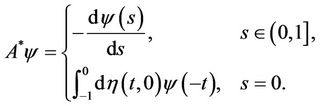
Define the linear operator  and the nonlinear operator
  by
by
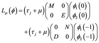 (15)
(15)
and
 (16)
(16)
respectively, where , and let
 .
.
By the Riesz representation theorem, there exists a 2 × 2 matrix function η(θ, μ), −1 ≤ θ ≤ 0, whose elements are of bounded variation such that
 for
for 
In fact, we can choose

where
 .
.
For  define
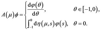 (17)
(17)
and
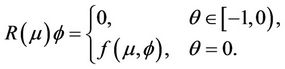 (18)
(18)
Then system (14) is equivalent to
 . (19)
For , define
 (20)
(20)
and a bilinear inner product
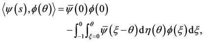 (21)
(21)
where η(θ) = η(θ, 0). Then A(0) and A* are adjoint operators. In addition, from Section 2 we know that ± are eigenvalues of A(0). Thus, they are also eigenvalues of A*. Let q(θ) is the eigenvector of A(0) corresponding to
  and
and  is the eigenvector of A* corresponding to
 .
.
Let 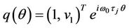 and
and .
.
From the above discussion, it is easy to know that 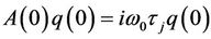 and
and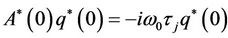 . That is
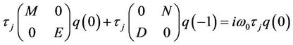
and
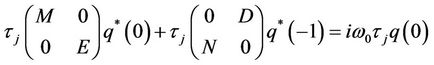
Thus, we can easily obtain

 .
.
Since

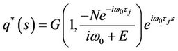
We may choose  and G as
 (22)
(22)
which assures that 
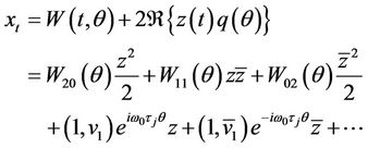
Using the same notations as in Hassard, Kazarinoff, and Wan [23], we first compute the coordinates to describe the center manifold  at μ = 0. Let
  be the solution of Equation (14) when μ = 0. Define
 (23)
(23)
On the center manifold  we have
 , where
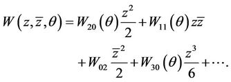 (24)
(24)
z and  are local coordinates for center manifold
in the direction of  and
and . Note that W is real if
  is real. We consider only real solutions. For solution
  of (14), since μ = 0,
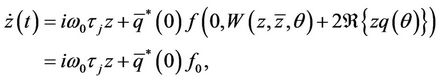 (25)
(25)
that is
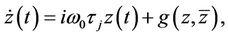 (26)
(26)
where
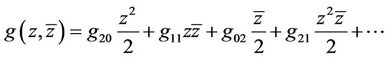 (27)
(27)
Then it follows from (23) that
 (28)
(28)
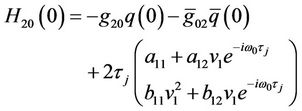
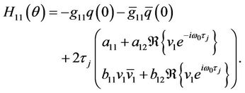
It follows together with (16) that
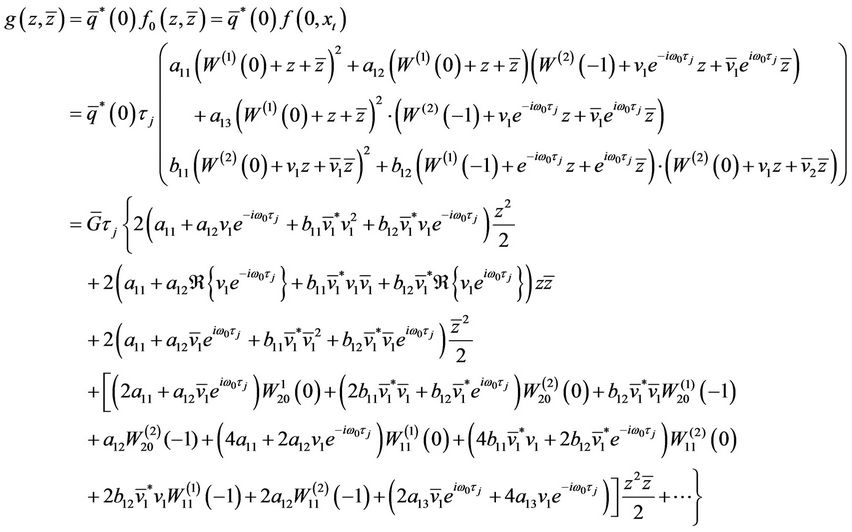
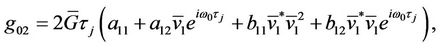
Comparing the coefficients with (27), we obtain
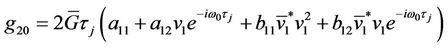 ,
,
 ,
,
Since there are  and
and  in
in , we still need to compute them.
From (19) and (23), we have
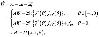 (29)
(29)
where
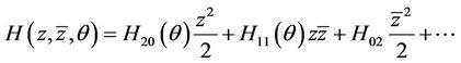 (30)
(30)
Substituting the corresponding series into (29) and comparing the coefficients, we obtain
 (31)
(31)
From (29), we know that for ,
,
 (32)
(32)
Comparing the coefficients with (30) gives that
 (33)
(33)
and
 (34)
(34)
From (31) and (33), we get

Note that , hence
 (35)
(35)
Similarly, from (31) and (34), we have

and
 (36)
(36)
In what follows we shall seek appropriate  and
and .
.
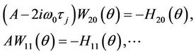
From the definition of A and (31) that
 , (37)
and
 (38)
(38)
where . From (29), we have
 (39)
(39)
 (40)
(40)
Substituting (35) and (39) into (37), and noticing that

and
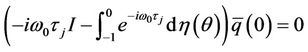 We obtain
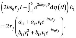 (41)
(41)
which leads to
 (42)
(42)
Therefore,
Similarly, substituting (35) and (40) into (38), we get
 (43)
(43)

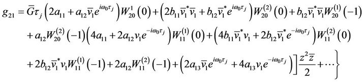
It follows from (35), (36), (42), and (43) that g21 can be expressed. Thus, we can compute the following values:
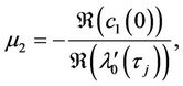

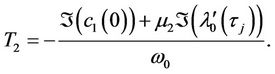
which determine the quantities of bifurcating periodic solutions at the critical value . That is,
  determines the directions of the Hopf bifurcation: If
  (
( ), then the Hopf bifurcation is supercritical (subcritical) and the bifurcating periodic solutions exist for
  (
( );
); determines the stability of the bifurcating periodic solutions: the bifurcating periodic solutions in the center manifold are stable (unstable) if
  (
( ); and
  determines the period of the bifurcating periodic solutions: the period increase (decrease) if
  (
( ). Further, it follows from Lemma 2.2 and (44) that the following results about the direction of the Hopf bifurcations hold.
Theorem 3.1. Suppose that (H1), (H2) hold. If  (
( ), then system (6) can undergo a supercritical (subcritical) Hopf bifurcation at the positive equilibrium
  when τ crosses through the critical values
 . In addition, the bifurcated periodic solutions occurring through Hopf bifurcations are orbitally asymptotically stable on the center manifold if
 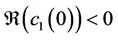 and unstable if
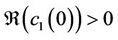 .
.
4. Numerical Simulations
In this section, we give some numerical simulations for a special case of system (6) to support our analytical results in this paper. As an example, we consider system (6) with the coefficients ,
,  ,
,  ,
,  ,
,  ,
,  ,
, ; that is
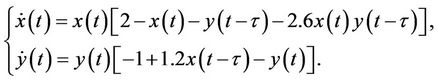 (45)
(45)
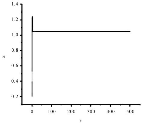
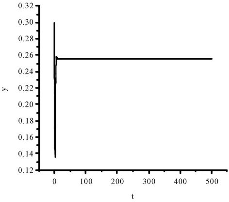
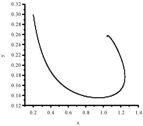
Figure 1. The numerical approximations of system (45) when τ = 0. The positive equilibrium E(1.04678, 0.25613) is asymptotically stable.

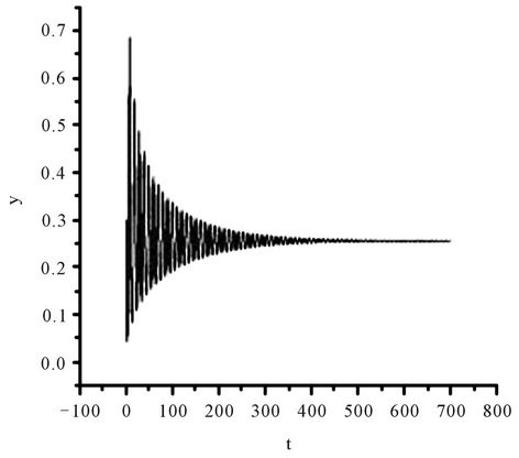

Figure 2. The numerical approximations of system (45) when τ = 1.35. The positive equilibrium E(1.04678, 0.25613) is asymptotically stable.
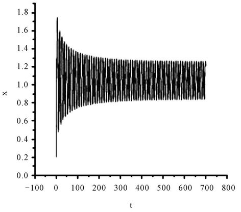
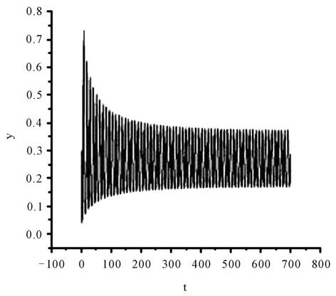

Figure 3. The numerical approximations of system (45) when τ = 1.4. The positive equilibrium E(1.04678, 0.25613) is unstable and a stable periodic solution bifurcates from E.
Obviously, (H1)  holds; therefore, system (45) has a unique positive equilibrium E(1.04678, 0.25613). From Lemma 2.1, we know that the positive equilibrium E(1.04678, 0.25613) system (45) is asymptotically stable when τ = 0; see Figure 1.
On the other hand, since (H1) , (H2)
  = −1.2342 < 0, from Theorem2.3, we know that the positive equilibrium E(1.04678, 0.25613) of system (45) is asymptotically stable when 0 ≤ τ < τ0 = 1.3788 and unstable when τ > τ0 = 1.3788, and system (45) can also undergo a Hopf bifurcation at the positive equilibrium E(1.04678, 0.25613) when τ crosses through the critical values
  = 1.3788 + 3.3502jπ (j = 0, 1, 2, ∙∙∙), i.e., a family of periodic solutions bifurcate from E(1.04678, 0.25613) see Figures 2 and 3.
5. Acknowledgements
The authors of this paper express their grateful gratitude for any helpful suggestions from reviewers and the partial support of Yunnan Provience science fundation 2011FZ086.
REFERENCES
- A. J. Lotka, “Elements of Physical Biology,” Williams and Wilkins, New York, 1925.
- V. Volterra, “Variazionie Fluttuazioni del Numero d’Individui in Specie Animali Conviventi,” Mem. Acad. Licei, Vol. 2, 1926, pp. 31-113.
- M. Brelot, “Sur le Probleme Biologique Hereditaire de Deux Especes Devorante et Devore,” Annali di Matematica Pura ed Applicata, Vol. 9, No. 1, 1931, pp. 58-74. doi:10.1007/BF02414092
- L. Chen, “Mathematical Models and Methods in Ecology,” Science Press, Beijing, 1988.
- Y. Song and S. Yuan, “Bifurcation Analysis in a Predator-Prey System with Delay,” Nonlinear Analysis: Real World Applications, Vol. 7, 2006, pp. 265-284. doi:10.1016/j.nonrwa.2005.03.002
- T. Faria, “Stability and Bifurcation for a Delayed Predator-Prey Model and the Effect of Diffusion,” Journal of Mathematical Analysis and Applications, Vol. 254, No. 2, 2001, pp. 433-463.
- S. Ruan, “Absolute Stability, Conditional Stability and Bifurcation in Kolmogorov-Type Predator-Prey System with Discrete Delays,” Quarterly of Applied Mathematics, Vol. 59, 2001, pp. 159-172.
- X. P. Yan and Y. D. Chu, “Stability and Bifurcation Analysis for a Delayed Lotka-Volterra Predator-Prey System,” Journal of Computational and Applied Mathematics, Vol. 196, No. 1, 2006, pp. 198-210.
- X. P. Yan and C. H. Zhang, “Hopf Bifurcation in a Delayed Lokta-Volterra Predator-Prey System,” Nonlinear Analysis, Vol. RWA 9, 2008, pp. 114-127. doi:10.1016/j.nonrwa.2006.09.007
- Y. Song and J. Wei, “Local Hopf Bifurcation and Global Periodic Solutions in a Delayed Predator-Prey System,” Journal of Mathematical Analysis and Applications, Vol. 301, 2005, pp. 1-21. doi:10.1016/j.jmaa.2004.06.056
- X. P. Yan and W. T. Li, “Hopf Bifurcation and Global Periodic Solutions in a Delayed Predatorprey System,” Applied Mathematics and Computation, Vol. 177, No. 1, 2006, pp. 427-445.
- J. Zhang and B. Feng, “Geometric Theory and Bifurcation Problems of Ordinary Differential Equations,” Beijing University Press, Beijing, 2000.
- S. A. Gourley, “Travelling Fronts in the Diffusive Nicholsons Blowflies Equation with Distributed Delays,” Mathematical and Computer Modelling, Vol. 32, 2000, pp. 843-853. doi:10.1016/S0895-7177(00)00175-8
- J. K. Hale, “Theory of Functional Differential Equations,” Spring-Verlag, New York, 1977. doi:10.1007/978-1-4612-9892-2
- J. Wu, “Theory and Applications of Partial Functional Differential Equations,” Springer-Verlag, New York, 1996. doi:10.1007/978-1-4612-4050-1
- C. H. Zhang, X. P. Yan and G. H. Cui, “Hopf Bifurcations in a Predator-Prey System with a Discrete Delay and a Distributed Delay,” Nonlinear Analysis, Vol. RWA 11, 2010, pp. 4141-4153. doi:10.1016/j.nonrwa.2010.05.001
- X. Z. He, “Stability and Delays in a Predator-Prey System,” Journal of Mathematical Analysis and Applications, Vol. 198, No. 2, 1996, pp. 355-370.
- Z. Lu and W. Wang, “Global Stability for Two-Species Lotka-Volterra Systems with Delay,” Journal of Mathematical Analysis and Applications, Vol. 208, No. 1, 1997, pp. 277-280.
- E. L. Rice, “Allelopathy,” 2nd Edition, Academic Press, New York, 1984.
- J. M. Smith, “Models in Ecology,” Cambridge University, Cambridge, 1974.
- J. Chattopadhyay, “Effects of toxic Substance on a TwoSpecies Competitive System,” Ecological Modelling, Vol. 84, 1996, pp. 287-289. doi:10.1016/0304-3800(94)00134-0
- A. Mukhopadhyay, J. Chattopadhyay and P. K. Tapaswi, “A Delay Differential Equations Model of Plankton Allelopathy,” Mathematical Biosciences, Vol. 149, No. 2, 1998, pp. 167-189.
- B. D. Hassard, N. D. Kazarinoff and Y. H. Wan, “Theory and Applications of Hopf Bifurcation,” Cambridge University Press, Cambridge, 1981.
- Y. Song, M. Han and J. Wei, “Stability and Hopf Bifurcation on a Simplified BAM Neural Network with Delays,” Physica D, Vol. 200, 2005, pp. 185-204. doi:10.1016/j.physd.2004.10.010