 International Journal of Geosciences, 2012, 3, 972-991 http://dx.doi.org/10.4236/ijg.2012.325098 Published Online October 2012 (http://www.SciRP.org/journal/ijg) The Theory and Application of Upwind Finite Difference Fractional Steps Procedure for Seawater Intrusion Yirang Yuan, Hongxing Rui, Dong Liang, Changfeng Li Institute of Mathematics, Shandong University, Jinan, China Email: yryuan@sdu.edu.cn Received August 14, 2012; revised September 10, 2012; accepted October 12, 2012 ABSTRACT Numerical simulation and theoretical analysis of seawater intrusion is the mathematical basis for modern environmental science. Its mathematical model is the nonlinear coupled system of partial differential equations with initial-boundary problems. For a generic case of a three-dimensional bounded region, two kinds of finite difference fractional steps pro- cedures are put forward. Optimal order estimates in norm are derived for the error in the approximation solution. The present method has been successfully used in predicting the consequences of seawater intrusion and protection projects. 2 l 2 l Keywords: Seawater Intrusion; Three-Dimensional Region; Upwind Fractional Steps; Norm Estimate; Numerical Simulation 1. Introduction Seawater intrusion refers to the invasion of salt water into the groundwater in coastal areas caused by the changes in natural water environment and social and economic development. In recent years, it has occurred in many countries in the world such as USA, Netherlands, Israel and Japan. After 1970s, the northern coastal area of our country, especially economic zones around Bohai such as Shandong, Hebei and Liaoning, is getting more and more seriously affected by this problem with Shan- dong province standing out. It leads to the great decrease in industrial and agricultural production, making people’s living conditions, especially their drinking water, poorer and poorer. Therefore, it is urgent that seawater intrusion be completely tackled. The mathematical model consists of water head equa- tion and salt concentration equation. Because of the compressibility of porous media and that of the fluid, the change in fluid density with the salt concentration, and with the consideration of the fact that the salt is in the moving state in porous media, there may occur convec- tion-dominated diffusion. While water is moving in the water-bearing stratum, it carries salt. The movement of this solute with underground water is called solute con- vection. Since salt is inhomogeniously distributed in the whole solution, it always diffuses from places with high- er concentration to places with lower concentration even if the solution does not move. 1.1. Water Head Equation With Darcy’s law, Euler method and Huyakorn’s lin- earization method, the water head equation is obtained [1,2]. 3 0 ,,,,0,, s T H SKHc tcqxyztJT t e (1) where S is the specific retention, 0 pgz is water head function, p stands for pressure, 0 repre- sents the density of reference water (fresh water), g is gravitational acceleration, z is the height of water con- taining layer, is density and depends only on the concentration of salt c, Hugakorn’s linearization 1 0 cc is adopted. cs is the concentration corresponding to the maximum density, and is the density difference ration 00s . Kg , is viscosity of the fluid, c is the density coupling coefficient. e3 = (0,0,1)T, is the porosity, q is source or sink term, and the permeability is noted by 1 2 3 00 00. 00 K KK K Cl 1.2. Salt Concentration Equation dissolved in the fluid causes The movement of C opyright © 2012 SciRes. IJG  Y. R. YUAN ET AL. 973 convection and diffusion of in porous media. From Fick’s law and mass conservation law we have the fol- lowing concentration Equation [1,2]. Cl T ,,,, , Dc c cxyzt J 0 * c t qC u Cl* C (2) where c stands for the concentration of , is the salt concentration near the source well. Darcy’s velocity and the diffusion matrix are denoted by 3 0 Hc ue 12 13 22 23 32 33 . DDD DD DDD , ,,,0 , ,,. and 11 21 31 DD 1.3. Initial Boundary Value Conditions To make a complete system, appropriate initial boundary value conditions are necessary in addition to the above equations. The initial value condition is ,0 0 0 ,, ,, ,, xyH xyz cxyz z ,t cxyz xyz 1 ,, , . yzt (3) There are three kinds of boundary value conditions. When concentration and water head are known, the first kind of boundary value condition can be given as ,,,,, ,, ,,, ,,, H xyzhxyztcx xyztxyzt J 2,ztJ 0, Dc (4a) The second kind of boundary value condition can be given to non-flow boundary: 0,, ,xy un n (4b) where n is the unit vector in outer normal direction. A kind of Stefan boundary condition is for free surface boundary. The boundary condition of water heat equation: Hz 3 3 ,,, 10,, ,,. xyz H zxyztJ t uw ',c c wn Cl 2 l ,, Dc xyz (4c) The boundary condition of salt concentration equation: 0 3 1 , .t J nu where w is the permeated fluid flow rate in a unit area and c′ is the concentration of in permeated fluid. In the study of seawater intrusion miscible model, for the miscible fluid Henry suggested an analytic solution under the simplified boundary condition and with the steady-state flow in the homogeneous medium [3]. Segol, Pinder, Grug, Heinrich and others studied the two- dimensional cut plane problem [4,5], and Huyakorn, Gupta and Yapa studied the solving process of the three- dimensional problem [5,6]. However, their calculations are made in specifically assumed conditions; therefore, they can not truly reflect seawater intrusion. For plane incompressible two-phase displacement which is assumed to be -periodic, Jim Douglas, Ewing, Russell, and others have published famous papers on the characteristic finite difference method and finite element method to solve the convection-dominated dif- fusion problems with finite difference method, and to overcome oscillation and faults likely to occur in the traditional methods [7-12]. For compressible two-phase displacement problem, Douglas and others have con- tributed much to the mathematical model of “infinitesi- mal compressibility”, numerical method and analysis [13-16]. Douglas and Yuan discarded periodic conditions, put forward a new modified characteristic finite dif- ference method and finite element method, and obtained optimal order estimation in norm [17-20]. Special treatment is needed for characteristic lines because the method of characteristics asks for interpolation and they may go through the boundaries near the solution regions. It is necessary to find out the intersection point of cha- racteristic lines and mesh boundaries and calculate their corresponding functional values. While such calculation is designed, we must determine whether characteristic lines really go through the boundaries in order to decide whether time steps lengths should be changed. In a word, the practical calculation is quite complicated [19,20]. For the convection-dominated diffusion problems, Axelsson, Ewing, Lazarov and others proposed upwind finite difference method [21-23] to overcome oscillation and to avoid computation complexity of the characteristic differential method near boundary meshes. Douglas and Peaceman applied the alternating-direction method to numerical reservoir simulation [24,25]. By using Fourier analysis, they succeeded in proving the stability and con- vergence according to the constant coefficient [26,27]. This paper, starting from the actual case, puts forward the modified method of upwind with finite difference frac- tional steps procedure for seawater intrusion. It can over- come oscillation and diffusion and computative comp- lexity. At the same time it can convert a three-dimen- sional problem into three successive one-dimensional problems, reducing computation complexity and making computation practical. Moreover, it increases the space calculation accuracy to the second order. Some tech- niques, such as calculus of variations, energy method, operator-splitting, upwind method, commutative law of Copyright © 2012 SciRes. IJG  Y. R. YUAN ET AL. IJG 974 2 l 2. The Upwind Finite Difference Fractional Steps Procedure multiplication of difference operators, decomposition of high order difference operators, the theory of prior estimates and techniques are adopted. Optimal order estimates in norm are derived to determine the error in the approximate solution. Thus the difficult problem has been solved [16,28]. For brevity we consider only the first kind of boundary value problem and the diffusion matrix ,,Dxyz of diagonal form. In order to get the solution by using finite difference method we use mesh region h instead of region Generally, this is a positive definite problem: Copyright © 2012 SciRes. *2 2 * ** 0, 0,,,,0 ii KKcK Kct DDxyztD * ** ,1,2,3, ,,, Ki xyz (5) . On space (x, y, z), let step lengths be h3, xi = ih1, yj = jh2, zk = kh3, where * , * , , are constants. * Our assumptions on the regularity of the solution of (1)-(5) are denoted collectively by * 1, 1, 2 , ,. W W LL 4, 222 ,HcL W Ht ct In this paper and express general positive constant and general positive small constant respectively, and have different meanings. 12 12 12 ,, ,,,, . ,, hijk ijk iijk yzjikj jik kijk kij Let h h n ijk W stands for the boundaries of , Xijk = (ih1, jh2,kh3)T, tn=nΔt, W(Xijk, tn) = . Let ,1,,1, 1/2, ,,1,,,1, ,1/2, ,,1,,1 ,1/2 ,,2, ,,2 ,,2, nnn hijkh ijkijkh ijk ijk nnn hijkhijki jkhi jk ij k nnn hijkh ijkij kh ijk ij k KCKX CKXC KCKX CKXC KCKX CKXC , 1211 11 1,1,,,,1, 1/2, , nnnnnn n xhxhhh ijkh ijkh ijkhijk ijk ijk KCHh KCHHHH (6a) 11 11 2,,1,,,,1 ,1/2 , nnnn n hyhh ijkh ijkh ijkh ijk yijk KCKCHHH H 12 () nn h ijk H h (6b) 1111 3,,1,,,,1 ,1/2 , nnnn n zhzhhijkh ijkh ijkh ijk ij k KCKCHHH H 12nn hijk H h (6c) 1111 . n nn nnn hxhhyhhzh xyz ijkijk ijk KC HKCHKC H nn hhh ijk KC H , n h ijk H and , n h ijk C be ,n ijk (7) 2.1. The Second Order Upwind Finite Difference Fractional Steps Scheme Let the finite difference solu- tions of n t n n h , ijk cX Xt and , respectively. If the finite difference solutions h and C are known, we find the finite difference solutions C, First, compute the approximate Darcy’s velocity as follows: 1n h1n h at tn+1. 123 ,, T n nnn U UUU 11 ,1, ,, ,1, 11 1/2, 1/2, , nn nn nn hh h ijkh ijkh ijkh ijk nn hh ijk ijk KC HH HH hh CC 0 12 nKC U 22 ,, 1,, 0 2 ,1/2, ,1 2 nn nn hh h ijkh ijk n nn hh ij kij KC KC HH UCC ,,,1, 22 /2, , nn h ijkh ijk k HH hh 33 ,, 1, 0 32 nn nn hh h ijkh ijk n nn hh KC KC HH UCC ,,, 1 33 , 1/2, 1/2 . nn h ijkh ijk ij kij k HH hh For salt concentration Equation (2), the modified method of upwind with finite difference fractional steps  Y. R. YUAN ET AL. 975 scheme is given by 3 1/3 , , n nn xh ijk nn yh ijk nn zh ijk n h ijk z C C C C 2 ,,iijk 1,, ijk h X 12 1/3 ,, , 1 1 111 1 1 1 222 2 1 1 333 3 ,, ,, *, , 12 12 12 nn nn h ijkh ijk n hijk x ijk y ijk Z ijk nn h ijkh ijk Ux UyU nn ijkh ijk CC Ct hUD D hUDD hUD D CC qC C ,1 ,, n h ijkijk (8a) 1/3 , nn h ijkijk Cg (8b) where 0i CD ,,1,2,3. i Di 2/3 1/3 ,, , 1 12/3 222 2 12 1, 2 (, )(, ), nn h ijkh ijk n hijk nnn yh h yijk ijk CC Ct hUDD CC jikj jik 2/3 1 ,,, nn h ijkijkijkh CgX (9a) (9b) 12/3 ,, , 1 11 333 3 12 1, 2 ,,, nn h ijkhijk n hijk nnn zh h zijk ijk CC Ct hUDD CC kijk kij 11 ,,, nn h ijkijkijkh CgX (10a) (10b) where 11, , nijk ijk Ux c U11 1,1,1/ 2,1,1,1/ 2, 1, 1, 1, nn n ijk ijkijk ijk ijkijkxijk x HUDDHUD Dc 2 11 2,2, ,1/2,2,2, ,1/2, 2, 2,2, ,1, nnn n ijk ijkijk ijk ijkijkijkijky ijk y Uy cUHUD DHUDDc 3 11 3, 3,,1/23,3,,1/2 3, 3,3, ,1, nnn n ijkij kijkij k ijkijkijkijkz ijk z Uz c UHUDDHUDDc and 1,0, . 0, 0. z Hz z 12/3 ,, , 1 3 12 , ,,, nn hijk hijk s ijk nnn hz hh zijk HH St KCHH kijk kij 11 ,,. nn h ijkijkijkh HhX Next, for fluid Equation (1) the fractional steps sinite difference scheme is given by , ,, 0 1/3 ,, 1/ 3 ,1 23 1 ,, ,, nn h ijkh ijknn sijkhx h xijk nn nn hyh hzh yz ijk ijk n nn h ijk h ijkh ijkn ijk ijk nn HH SKCH t KCHKC H C CC q t KCCijkii jk 31 2hh zijk 1/3 1 ,,, nn h ijkijkijkh HhX (11a) (11b) 2/3 1/3 ,, , 2/3 2 12 , ,,, nn h ijkhijk s ijk nn n hy hh ijk HH St KC HH kjjik 2/3 1 ,,, nn h ijkijkijkh HhX y ji (12a) (12b) (13a) (13b) The initial approximation reads 00 ,0, 0 ,, h ijkijkh ijkijkijkh CcXHHXX . , nn CH n t (14) The algorithm for a time step is as follows: Assuming the Approximate solution ,,hi jkhijk at time is known, it is needed to find out the approximate solutions at the next time level. First, compute Darcy’s velocity n U, from schemes (8a), (8b), and method of speedup is used to get the solution of transition sheaf 1/3n C 2/3n C ,hijk along x direction. Secondly, from schemes (9a), (9b) we obtain the solution of transition sheaf ,hijk . Thirdly, from schemes (10a), (10b) we obtain solution 1n C 1/3n H ,hijk . Next, from (11a), (11b), by using method of speedup, we get the solution of transition sheaf ,hijk along x direction; from (12a), (12b) we obtain the solution of transition sheaf 2/3n H ,hijk . Finally, from schemes (13a), (13b) we obtain solution 1 , n h ijk H. So a complete time Copyright © 2012 SciRes. IJG  Y. R. YUAN ET AL. 976 step can be taken. At last, it is because of the positive condition that this finite difference solution exists, being the sole one. 2.2. The First Order Weighted Upwind Finite Difference Fractional Steps Scheme For salt concentration Equation (2), the first order up- wind finite difference fractional steps scheme is given by 12 1/3 ,, , 23 ,, ,, *, ,,1 ,, nn nn h ijkh ijk n hijk x yh z yZ ijk nn Ux Uy h ijkh ijk nnn ijkh ijkh ijk CC t DCD CC qCCi jk 3 1/3 1 , , 2 ,, n n x hijk nn h ijk n Uz h ijk CD C C C i ijk 1,, ijk h X (8a)′ 1/3 , nn h ijkijk Cg (8b)′ 2/3 , n hijk D CC 2/3 1,, nn ijk h X 2/3 1/3 ,, 2 , 12 ,, , nn h ijkh ijk nn hijkyh y CC C t jikj jik (9a)′ ,hijk ijk Cg (9b)′ 12/3 1, nn nnn hh ijk CC DCC 11 ,,, nn h ijkijkijkh CgX ,, 3 , 12 ,, , hijkh ijk h ijkz z C t ki jk kij (10a)′ (10b)′ where 1,1, 1,1, 1 1 , nnn n Ux ijkijkijkijkx ijk cUHUHUc h 1, 1, 1, 12 x nijk i jki jk Uc c and 23 ,, , nn Uy Uz ijk ijk cc are defined similarly with a con- stant 0, 1 3 0,1 , . The algorithm is similar to that of Scheme (8)-(13). 3. Convergence Analysis For brevity we assume 1,hN T ijk ,, , ih,tnt ,nn WX tWjh khn , ijk ijk . Let hh π, HcC where H and c are the exact solutions of this problem (1) - (5), and Hh and Ch are the difference solutions of the schemes (8) - (13). ,, and 1 denote the inner product and the norms on the dis- crete spaces l2(Ω) and h1(Ω) corresponding to L2(Ω) and H1(Ω) [19,20,29]. First consider the second order scheme. Theorem I. Suppose that the exact solutions of prob- lem (1)-(5) satisfy condition: Adopt the modified method of upwind procedures (8)- (13). Let the dissectible satisfy relation: 2 tOh . Then the following error estimates hold: 1, 1,4, 2 ,, ,. Hc WWL W 4, 22 2 ,, tctLWHt c t LL 2 11 2 22 (; )(; ); *2 (;) hhth LJhLJh Jl th LJl HHcC dHH dcCM th (15) where 2 2 ;; 0 sup ,sup N nn LJS LJS SS ntTNtT n gg gt * . depends on , Constant c 1/3n C2/3n h C and their derivatives. Proof. First consider the concentration equation. For Equations (8)-(13), dispel h and , and we get the following equivalent form: 123 1 11 ,, 1 11 ,1 1 11 22 2 1 11 33 3 ,,,, ,, , 12 12 12 nnn nn h ijkh ijk nnn hijkx h xijk ijk nn yh yijk ijk nn zh Zijk ijk nnnn h ijkh ijkhijkijkh Ux Uy Uz CC h CUDDC t hUDD C hUDD C CCCqC *, , 1 1 21 11 1 1 1 22 2 1 11 11 1 1 1 33 3 1 2 2 12 1|| 2 12 12 12 nn ijkh ijk nn xh x ijk nn yt h y ijk nn xh x ijk nn zt h z ijk n ijk C h tUDDC hUD DdC hUD D C hUDDdC hUD 1 1 1 1 1 33 3 1 1 3 1 1 1 1 1 122 2 1 1 133 3 12 1|| 2 12 1, 2 1,, n yh y nn zt h z ijk n x ijk nn xh y y nn n hzth z ijk DC hUDDdC h tUD h DCUDD h CUDDdC ijkN 1, (16a) Copyright © 2012 SciRes. IJG  Y. R. YUAN ET AL. Copyright © 2012 SciRes. IJG 977 11 , , ijk ijkh X 1n . (16b) nn h ijk Cg From Equation (2) (tt) and (16) we have the concentration error equations. 1 11 22 11 1 ,, 1 11 ,1 11 11 11 223 3 23 1 ,, ,, , 12 11 22 nn n nn hijk hijk nnn hijkx h xijk ijk nnnn yh zh yZ ijk ijk ijk ijk nn n h ijkijkh ijk Uxu xUyu h CUDD t hh UD DUDD Cc C 11 33 11 , ,,, 11 11 11 111 11 11 11 11 222 22 11 22 11 22 12 nnn nnn ijkh ijkijk yUzuz nnn xh xijk ijk ijk nnn yh yijk ijk ijk cCc hh uDUD DC hh uDUD DC h 11 11 11 333 33 1*, 1*, ,,, 11 11 21111 11 22 12 12 11 22 nnn zh zijk ijk ijk nnnnnn ijkh ijkijkijkh ijkh ijk nnn xy xy ijk h uDUD DC qC cqCC hh tuDDcuDDd n t c 11 11 1 11 22 12 11 11 111 11 22 12 11 22 11 22 nn nn xh yth xy ijk ijk nnn xy xy ijk ijk hh UDDCUDDdC hh uDDcUD DdC ijk n th 11 11 31111 11 22 12 11 11 133 1 31 1 1 1 12 2 {1( (1( 22 11 22 1|| 2 nnn xy xy ijk nnn zt zx ijk ijk nn xh hh tuDDc uDD hh uD DdcUD h DCUD 11n c 1 1 1 23 3 1 31, 1|| 2 ,1,,1, nn yh y nn zt hijk zijk h DC UD DdC ijkN (17a) 10, , n ijkijk h X (17b) where 12 . 1, nijk th 1/3n h H2/3n h H Next, consider the fluid equation. For Equations (11)-(13), dispel and , and we get the following equivalent form:  Y. R. YUAN ET AL. 978 1 ,, 11 ,12 1 , ,, 3 0 21 12 1 13 nn h ijkhijknn nn sijkhxhhyh xy ijk ijk n nn h ijk h ijkh ijknnn ijkijkh h zijk nnn hxs hyth xy ijk nn hxs hzth xz HH SKCHKCH t C CC qKCC t tKCSKCdH KCSKC dH 1 3 nn hzh z ijk KCH 1 23 311 123 ,1 nn hys h yz ijk nnnn hxshys hzth xyz ijk KCSKC tKCSKCSKCdH , ,1, nn zthijk dH ijkN 11 ,. nn ijk h HhX 1n (18a) ,hijk ijk (18b) From Equation (1) (tt) and (18) we have the fluid error equations. 1 1 , 11 1 00 11 33 nn nn ijkh ijk ijk ijk nnnn hhhijkijk ijk nn nn hh zz ijk ijk cC Kc KCHq t Kc cKCC 1 111 ,1 2 3 ππ πππ nn ijk ijknnnn nn sijkhxhy hz xy z ijkijk ijk n ijk SKCKCKC t q 2111 12 11 12 1 11 13 2 1 23 nnn xs yt xy ijk nnn n hxs hythxs xyx z ijk nnn n hxs hzthys xzy z ijk nn hys hz yz tKcSKcdH KCSKC dHKcSKc KCSKC dHKcSKc KCSKC 11 3 11 3 nn zt ijk nn zt ijk dH dH 31111 1 123 11 123 2 , 1,,1, n th ijk nnnn xsys zt xyz ijk nnnnn hxshys hzthijk xyz ijk dH tKcSKcSKcdH KCSKCSKC dH ijk N 1 , 1 π0, , n ijkijk h X (19a) (19b) where 12 2, . nijk th We shall introduce the induction hypothesis: 1, 1, ,0,,0, nn ht 0 sup maxπ nL (20) where 22 2 1, 0,0, ππ π,. nn n h 11 πππ nnn t ijkijkijk We consider fluid error Equation (19). Test error Equa- tion (19) against and summing it up y parts, we have b Copyright © 2012 SciRes. IJG  Y. R. YUAN ET AL. 979 11 11 12 11 312 11 1 1 00 1 π,ππ,ππ,π 2 ()π,ππ,ππ, ,π,π ,π nnn nnn nn stthxxh yy nnnn nnnnn hzzhxxhyyh nnnn nn hhhttt nn h nnn t SddtK CKC KCKCKCKC KcKCHdtd dt cC qqdt 3 ππ,π n nn z z 11 33 211 1 12 1 12 31111 1 123 11 123 ,π ) ,π nnnn n hh t zz nnn xs yt xy nnnn hxshytht xy nnnn xsys zt xyz nnnn hxshyshzth xyz KccKCC dt tKcSKcdH KCSKC dHdt tKcSKcSKcdH KCSKCSKC dH 1 2 ,π, nn t dt π. n t dt (21) Now we estimate the terms on the right-hand side of (21). 11 22 ,π π, nnnn ht nn 2 hh ht cKC Mtt Hd t dt (22a) 22 ,π π, nn tt nn tt dd t dtdt (22b) 1 1 00 22 2 ,π π, nn h nnn t nn t cC qqdt ttd t (22c) 11 33 222 2 ,π π, nnnn n hh t zz nn n ht ccKCCdt ttd t (22d) For the fifth term on the right-hand side of (21). 31111 1 123 11 123 31 12 11 122 11 ,π π,π ,π nnnn xsys zt xyz nnnnn hxshyshzth t xyz nnnn hxshyt t xy nnnnn shytt xy x tKcSKcSKcdH 1 hx n CSKCSKCdHdt tKCSKCdd SKcKCdHd Kc KC KC (23) 11 2,π. nnnn hxsyt t y SKc dHd For the first term on the right-hand side of (23), though the operators K are self-co , xy xy K njugate, positive definite and bounded, space region is cubic. However, their products are generally incommutative. Noting that ,,,, xy yxxxy y yy xxxyyx we have Copyright © 2012 SciRes. IJG  Y. R. YUAN ET AL. 980 3 tK1 12 2 311 12 ,2 ,1 1/ 2,,1/ 2,,1/ 2,1/ 2, ,,1 1 ,1 2 1/ 2,,1/ 2, π π π()π π nnnn hxshyt t xy Nnn nnnn hhs ijkxytijkhys ijkhxtijk ijkijkijkijk ijk nn s ijkhxhytij ijkijk CSKCdd tKCKCS dKCSKCd SKCKCd 1 21 , , 1/2,1/2, 1 2,12 , 1/2,1/2,, 1/2, 13 ,1 1/2 , π ππ. nn nn khhxs ijkxytijk ij kijk nnn xhys ijkhh ij kijkijk nnn yx sijkhxt ijkyt ijk ijk KC KCSd KCSKCKC SKCdd h (24) From induction hypothesis (20) we learn that n KC , 1h, 2, h KC n 1 11 nn s h SKC are pression (24), the positive definite property of 1 12 ,, , xh y KC bounded. To the first and second terms of ex KS should be applied, and high-order difference term πn yt ijk d should be separated. By using Cauchy inequality to get ,1 ,12 1/2,,1/2, 21 , ,1/2, 1/2, ππ N t nn n ys ijkhhxhytijk ijk ijk nn hhxsi ij kijk SK CSKCKCd KC KCS eliminate the terms concerned, we can 2 2 ,1/ 2, πnn ijkh ijk KC 31 12 , 1/ 2,,1/ 2, ,, 1 {nn hhs ijkxy ijkijk ijk tKCKCSd 1/2, xt ijkd 11nn ijks ijk 12 3 132* 3 * ,, 1 22 1 1 ππ 2 π. N nn jkx y tijksx ytijk ijk nn h dhKStd h 1 22 2 3 32* 3 * ,, 1 1 ππ() ππ 2 N nn n xt ytsxytijkh ijk ddtKSt dhM For the third term of (24), we have t (25a) 1 2, 12 , 1/2,1/2,, 1/2, 13 ,1 1/2 , 22 1 ππ ππ. Nnnn hysijkhh ij kijkij k nnn yxsijkhxt ijkyt ijk ijk nn hh C SKCKC SKCdd h Mt (25b) Sim 3 ,, 1 x ij k tK ilarly, for the other terms, we can obtain 1 12 222 2 11 11 22 ,π ,ππ . nnnnn ythxshyt ht xy nnnnnn yszth h yz dH KCSKCdHd KcSKcdHMt t (26) Now, we consider the sixth term of the right-hand side of (21). 3111 12 nn xs xy tKcSKc 1 3 11 123 22222 4 2 3*3 1 * ,π 1πππ . 2 nn zt nnnnn hxshyshzth t xyz Nnnnn sxyztijkhh cdH KCSKCSKC dHd 411 11 12 nn xs ys xyz tKcSKcSK ,, 1ijk St dhMtt (27) Copyright © 2012 SciRes. IJG  Y. R. YUAN ET AL. 981 For the last term on the right-hand side of (21). 2 2. ntt From (21)-(28) we can obtain 22 11 2,πππ nnn n thh dtM (28) 2 *11 222222 14 1 ππ,ππ,π 2 ππ π. nnnnnnn hhhh nnnnn n hh hh Sdt KCKC 2 st h h t dhttdt (29) on error equation. Test err 11n ijk ijk Next, consider the concentrati or Equation (17) against nn t ijk and sum- ing it up by parts, we have 11 2 1 1 111 11 1 11 11 11 1 1 ,, , ,,1 2 , nn n nnnnnnn ht txx nn nnnn hth Ux UxUy h CddtDu D D Ccd C 1 11 2231 23 ,1 ,1 22 nn nnnn yy zz hh Du D uD 233 11 ,,, 11 11 11 111 11 11 11 11 111 22 1 11 3 ,, 11 , 22 11 , 22 12 nnn nnnnn tht UyUz Uz nnnn xxht nnnn yyht n cdC cdt hh uDuDDCd hh uDuDDC d huD 11 11 11 3 1*,11*, 11 11 311 11 31 13 4 1 1, 2 , 11, 22 12 nnn zzht nnn nnnn t nnnnn xx hzztt n huDD Cdt qCCqC Cdt hh tuDDCuDDdd h tu 1 1 1 11 11 11 13233 33 1 1 11, 22 , nnnn n xx hyyhzzt nn t D hh DCuDDCuDDd dt (30) First, we estimate the second term on the left-hand side of (30). 1 1 1 1 111111 11 11 1 ,1 ,1 2 nnnn nnn x hh DuD DuD (31a) 1 1 122 1 11 11 1 22 ,1 . 2 xx x nnn nn xxht h Du D Mtdt Copyright © 2012 SciRes. IJG  Y. R. YUAN ET AL. 982 Similarly, 1 1 111 22 2 11 11 11 111 2222 22 ,1 2 1,1 ,1 22 2 nnnn yy nn nnn nn yyyy h DuD hh DuDDuDM (31b) 22 . n ht tdt 1 1 111 33 3 11 11 11 111 3333 33 ,1|| 2 1,1 ,1 22 2 nnnn zz nnnnnnn zzzz h DuD hh DuD DuDM (31c) 22 . n ht tdt Now, we estimate the terms on the right-hand side of (30). In induction hyhesis (20) n U is bounded, so we have pot 1 11 22 2 1 11 ,, nn nnnnn n hth Uxu x CcdtMUu t 2 ,. n t tdt ilarly, (32a) Sim 11 22 33 11 ,, ,, ,, nn nn nnn nnn htht UyuyUzuz CcdCcdt 22 2 2 2 22 33. nn nn nn ht UuUutt dt (32b) For the second term on the right-hand side of (30), we have 11 11 11 111 11 11 11 2 11 333 33 11 , 22 11 , 22 nnnn xxht nnnnnn zzht hh uDUDDCd hh uDUDDC dtMuUt (33) 22 . n t t dt For the third term, we have 22 ). n tt t dt (34) We consider the fourth term, and we have 1* ,1 1*,2 ,( nnn nnnnn qCcqCCdtMt 11 11 3(1 2 hh tU 1 11 22 12 11 11 31 1,1/2,2, ,1/2,1,2, ,1, 2, ,, 1 1 , 2 11 22 nnnnn xhyt t xy Nnnn ijki jkijkijk h ijkijkijkx ijk DDCUDDdd hh tDDC UDUD 2 n d 11 11 1 2, ,1/2,2, ,1/2,2,1,2, ,1/2, ,2, 1, 1 11 1 1,1/2,2,1, ,2, 1, 11 22 11 22 ytijk nnn n i jki jkijkijki jk xh ijkijkijkytijk nn n i jkijkijk yh ijkijkijk hh DD C UDUDdD hh DCUD UD 1 3. nn xtijkxyt ijk ddh Copyright © 2012 SciRes. IJG  Y. R. YUAN ET AL. 983 On positive definite condition: * 1 1.C In induction hyhesis (20) n U is bounde *1 ** * ** * ,0 ,0 i DD DC pot d, so we have 1 1 0 12 n hUD b 0,1,2,3, 11 11 31 11 2 12 3 122 23 *2 ** 0 {1 1 22 . 2 2 , nnnnn xhyt t xy nnn xythtt hh tUDDCUDDdd tDbdMtdd 2 Thus, for the fourth term we can obtain 22 111 11 1 1111 11122 11 2 , 11 1 22 2 nnnnn yt t xy nnnn n xyt xy hh DDdd hh h uDUDDcuDDdc 11 11 31 11 12 11 22 xh tU DDCU 3 122222 2*21 1 ** 0 , . 2 n t nnnnn xyth h d tDbdM t (35a) Similarly, for the fifth and sixth terms we have 11 11 31 11 33 13 3 1222 2*2 ** 0 2222 11 11 22 2 . nnn xh zt xz nnn xyt xzt yzt nnnn hh hh tUDDCUDDd tDbd dd Mt , nn t d (35b) For the seventh term we have 1 1 1 11 2 12 1 1 1 233 3 4 222222 3*21 1 ** 0 22 1, 2 . 2 nn xx h nnn n yy hztt z ijk nnnnn xyzth h h CUD h DCUD Ddd tDbdM t (36) For the last term 1 1 411 n h tUDD 2 14 ,.Mth (37) For error Equation (30), from (31)-(37) we can obtain 2 1 nn n tt dtdt Copyright © 2012 SciRes. IJG 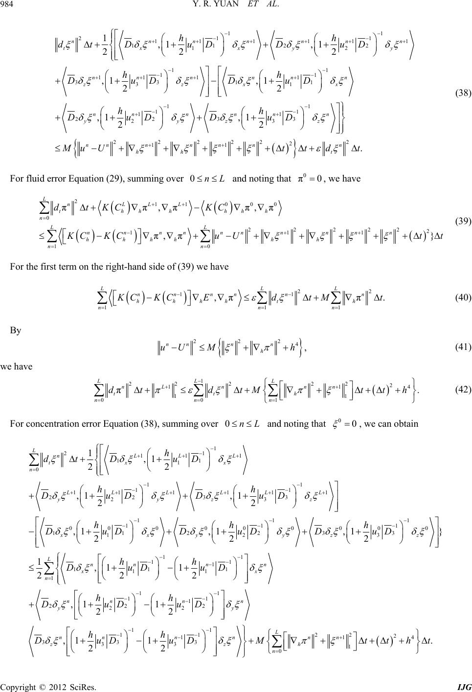 Y. R. YUAN ET AL. 984 11 11 1 1 2 1 2 nn y n x D 211 11 112 12 11 11 11 11 3311 3 1 1 1 22 2 1,1 ,1 22 ,1 ,1 22 ,1 2 nnnnn tx xy nn nnn zzx nn y hh dt DuDDu hh DuDDuD h DuD 1 1 1 33 3 22222 2 11 ,1 2 . nnn n yz z nnnnnnn hh t h DuD (38) 2 uUtt dt For fluid error Equation (29), summing over 0nL M and noting that 0 π0 , we have 000 0 22222 2 111 10 ππ,ππ,π π,π} th hhhhh n LL nnnnnn nnnn hhhhh h nn dtKCKC 211 LnL LL CKC uUtt (39) For the first term on the right-hand side of (39) we have 22 1 ππ. LLL n h n 11 11 , nnnn n hhhht nn CKC EdtM t (40) By 222 4, n hh (41) w nnn uU M e have 124 . LLL tth 22 222 11 11 001 πnL nnn tth nnn dt dtM (42) For concentration error Equation (38), summing over 0nL and noting that 0 0, we can obtain 1 21 11 11 1,1 LnLL h dt DuD 1 1 0 11 11 111 11 1 2233 23 11 11 00 000 0 112 2 12 22 ,1 ,1 22 ,1 ,1 22 L tx x n LLL LL L yyzz xxyy hh Du D DuD hh DuD DuD 1 11 11 1 11 1 11 1 11 11 1 1 33 3 1,1 1 222 ,12 Lnn nn xx n n nn z hh Du DuD hh h DuD 1 00 0 33 3 ,1 } 2 zz h DuD 1 22 2 22 ,1 1 22 nn n yy Du DuD 122 12 114 3 31 0 1. 2 L nn nn zh n huDMttht Copyright © 2012 SciRes. IJG 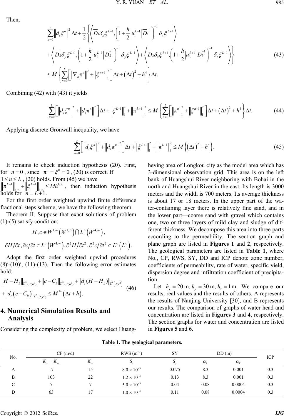 Y. R. YUAN ET AL. Copyright © 2012 SciRes. IJG 985 Then, 1 21 11 1 11 1 0 11 111 1 223 23 22 2 14 1 0 1,1 22 ,1 ,1 22 π. LnLLL tx x n LL L LL yyz Lnn h n h dtD uD hh DuDD Mttht 11 11 3 L z uD (43) Combining (42) with (43) it yields 24 .tht 22 2222 11 1 11 11 0 0 πππ L L nn LLnn tt n n ddt Mt (44) Applying discrete Gronwall inequality, we have 24 .Mth (45) It remains to check induction hypothesis (20). First, for 00 π0 , (20) is correct. If 1olds. From (45) we have 22 22 11 11 0 ππ LnnLL tt n ddt 0n, since nL, (20) h 11 1, LL 1/2 1, π h , then induction hypothesis r 1.nL For the first order weighted upwind finite difference fractional steps scheme, we have the following theorem. Theorem II. Suppose that exact solutions of problem (1)-(5) satisfy condition: 4, , holds fo 1, 1, ,Hc WWLW 2 , 4,22 2 ,, tctLWHt c t LL . Adopt the first order weighted upwind procedures (8 mates hold: )′-(10)′, (11)-(13). Then the following error esti 11 22 (; )(; ); ** () . hhth 22 (; ) JhLJhLJl HHcC dHH dcCM th (46) 4. Numerical Simulation Results and Analysis heying area of Longkou city as the model area which has 3-dimensional observation grid. This area is on the left bank of Huangshui River neighboring with Bohai in the north and Huangshui River in the ea meters and the width is 700 meters. Its average thickness is about 17 or 18 meters. In the upper part of the wa- ter-containing layer there is relatively fine sand, and in the lower part—coarse sand with gravel which contains one, two or three layers of mild clay and sludge of dif- ferent thickness. We decompose this area into three parts according to the permeability. The section graph and plane graph are listed in Figures 1 and 2, The geological parameters are listed in Table 1, where No., CP, RWS, SY, DD and ICP denote zone number, coefficients of permeability, rate of water, specific yield, dispersion degree and infiltration coefficient of precipita- tion. Let 20m, 30m, 1m. xyz hhh th LJ l Considering tp st. Its length is 3000 respectively. he comlexity of problem, we select Huang- We compare our results, real values and the results of others. A represents ults. The comparison of graphs of water head and concentration are listed in Figures 3 and 4, respectively. The section graphs for water and concentration are in Figures 5 and 6. olog ) SY DD (m) the results of Nanjing University [30], and B represents our res listed Table 1. The geical parameters. CP (m/d) RWS (m−1 No. ICP xyy K zz S S T A 17 15 8.0 10–5 0.075 8.3 0.001 0.3 B 103 22 1.2 0–4 0.13 8.3 0.001 0.3 C 7 7 5.0 –5 0.04 0.08 0.0004 0.3 0.11 0.08 0.0004 0.3 1 10 D 63 17 1.0 10–4 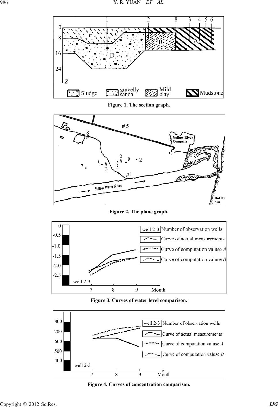 Y. R. YUAN ET AL. 986 Figure 1. The graph. section Figure 2. The plane graph. Figure 3. Curves of water level comparison. Figure 4. Curves of concentration comparison. Copyright © 2012 SciRes. IJG  Y. R. YUAN ET AL. 987 Figure 5. Sptember. ection graph of waterevel computation in Se l Figur ber. From the above we can see that the computation re- sults are exact, and the algorithm given in this paper is stable and can be used as the algorithm for the simulation of large-scaled problems. 5. Consequences of Protection Projects and Applied Modular Form of Project Adjustment 5.1. Consequences of Projection Projects The main water conservanc trusion include projects for water saving, Yellow River regulation, water retaining and artificial precipitation. Their ultimate goals are to increase water supplies and to decrease the extraction of underground water the produc- tion of human and animal needed, so that the descent of underground water level will be slowed down and even underground water be increased. All this is very effective. Up to now, the protection project results are mainly em- pirical and qualitative. We have not seen publications both in China and abroad about the real salt water and fresh water movement changes after the projects are si- mulated with computers. There uantitative and comprehensive predictions of vari- ous pr cts of water-saving project on seawater intrusion. Take the average precipitation amount in many years (Refer to “Comprehensive Control Plan Against Seawater Intrusion in Laizhou Bay Area of Shandong Province”). Simulate water levels and changes of salt concentration two months after the peak period (July-August) in the following four conditions: the pre- sent pumping out, saving water 10%, saving water 20% and saving water 30%. Water heads and concentrations of some wells at initial time are listed in Table 2. The calculation and comparison results are listed in Tables 3 and 4. The predictive sections saving 20% are From the above we can see the consequences of water saving projects are remarkable. During raining seasons the underground water level rises again quickly. In dry seasons, its descent is slowed down. So the projects slow down the migration of salt concentration to fresh water Table 2. The initial values of water head and concentration. Well No. Water head (m) Salt concentration (mg/L) e 6. Section graph of Cl‾ concentration in Septem y works against seawater in-listed in Figures 7 and 8. are no publications on the q ojects. Now we take watersaving project as an example to discuss the predictive result of the projects. Scheme: Keep the present precipitation level. Take into consideration the effe at water 1-2 –1.01 3667 2-2 –2.20 3000 3-2 –2.77 377 2.87 100 4-2 –3.10 400 5-2 –3.13 98 6-2 – Copyright © 2012 SciRes. IJG  Y. R. YUAN ET AL. 988 Table 3. The effects of water saving projects on water head. Well number, Water head Saving water 1-2 2-2 3-2 4-2 5-2 6-2 0 –0.45 –1.75 –2.04 –2.42 –2.32–2.16 10% –0.34 –1.52 –1.80 –2.14 –2.07–1.93 20% –0.23 –1.31 –1.56 –1.87 –1.81–1.71 30% –0.12 –1.10 –1.33 –1.60 –1.55–1.48 Table 4. The effects of water saving projects on salt concen- tration. Well number, Water head Saving water 1-2 2-2 3-2 4-2 5-2 6-2 0 3871 3044 1521 101 98 99 10% 3753 3088 1507 101 98 99 20% 3725 3032 1493 101 98 99 30% 3696 3027 1479 100 98 100 Figure 7. The water head prediction at 20% water saving in July-August. Figure 8. The salt concentration prediction at 20% water saving in July-Augu areas. 5.2. Predicting the Consequences of Underground dams and ith the aim to regulation ur water anrevseaer intrusion. Underground cut-off walls are built to stop undercnt aawelod the dam are l and are We can ae l ability of damhepcns the ing e. ds op undercurrent and increase water supply, playing the pitation supply coefficient, playing the role of retaining andg water. This dams in sead egiretain and regulate under- ground water, increase the heof the fresh water heads in upper vheseseater intrusid thyi iman fr invadedgions inweraches. Finally, the dam in loweres (ne pt seawattrn. Tidal es uomdwarte art on the ground and the underground base. Our both parts are very useful. The on-the-ground part prevents seawater coming in with windstorms, while the underground part prevents sea- water intrusion in common situations because of its small permeability. The advantages of tidal barrages especially obvious in of windy period. There usually are two kinds of anti-percolator, namely: lower reaches dam in seawater invaded region, and upper reaches dam in seawater invaded region. e sea, or in other places where both salt and esh water move freely. If a large amount of under- ground water is pumped out in coastal areas, water level goes down rapidly. When underground water level is lower than the average tidal level, seawater intrusion happens. This is because of the continuity between inland fresh water and seawater. Underground dams reduce greatly or completely stops the permeability of auto- chthonous layer. Therefore, cut-off walls can reduce the possibility of the seawater in lower reaches intruding trusion thanks to the combined actions of their own and ater curtain. Underground dams should be located far from the upstream of tides with the consideration of ould he built who undem. st. Underground Dam and Tidal Barrage Projects reservoirs are built w ndergoundd pent wat urrend seater, since water had is w an s safety ocated high. under the ground, so say th the stability epaget the scontro s is t key oint. Our pratice idicate followfour ffectsFirstly, undergroun dam st role of saving and regulating water. Secondly, they raise underground water level and increase artificial preci- supplyin awater inv rdly, the upper reache ed rons ight reaches, relie ing t prent wa on anus plang anportt roleor seawate re reach lo ear th re coast) s usiorevener in barragare usally cpose of to ps: th p analysis indicates that Lower reaches dams should be built on rivers which empty into th fr inland. Moreover, they can retain and regulate the drainage of underground water. They stop seawater in fresh w tide actions. Otherwise, tidal barrages sh se upper part is barrage and the lower part is rground da As for the upper reaches dams in seawater intruded areas, since the intrusion has occurred, the underground walls must be built at the head of these areas with the aim to retain underground water and increase the fresh water head from upper reaches and to make seawater intrusion stable. This is also useful for inland fresh water areas far from the coast because these dams prevent the decrease of fresh water amount going into the sea, and Copyright © 2012 SciRes. IJG 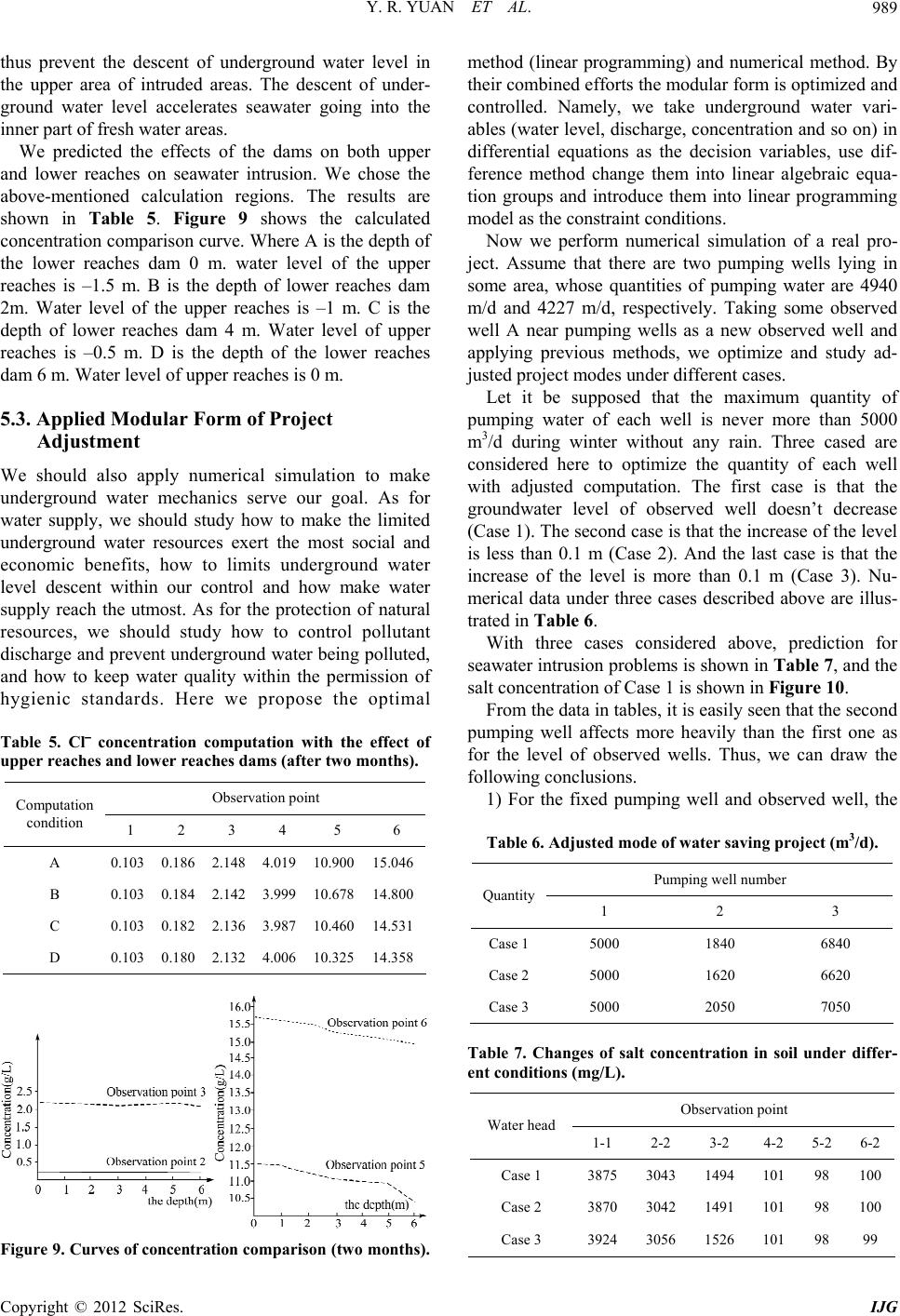 Y. R. YUAN ET AL. 989 thus prevent the descent of underground water level in the upper area of intruded areas. The descent of under- ground water level accelerates seawater going into the inner part of fresh water areas. We predicted the effects of the dams on both upper and lower reaches on seawater intrusion. We chose the above-mentioned calculation regions. The results are shown in Table 5. Figure 9 shows the calculated concentration comparison curve. Where A is the depth of the lower reaches dam 0 m. water level of the upper reaches is –1.5 m. B is the depth of lower reaches dam 2m. Water level of the upper reaches is –1 m. C is the depth of lower reaches dam 4 m. Water level of upper reaches is –0.5 m. D is the depth of the lower reaches dam 6 m. Water level of upper reaches is 0 m. 5.3. Applied Modular Form of Project Adjustment We should also apply numerical simulation to make underground water mechanics serve our goal. As for water supply, we should study how to make the limited underground water resources exert the most social and economic benefits, how to limits underground water level descent within our control and how make water supply reach the utmost. As for the protection of natural resources, we should study how to control pollutant discharge and prevent underground water being polluted, and how to keep water quality within the permission of hygienic standards. Here we propose the optimal Table 5. Cl‾ concentration computation with the effect of upper reaches and lower reaches dams (after two months). Observation point Computation condition 1 2 3 4 5 6 A 0.103 0.186 2.148 4.019 10.900 15.046 B 0.103 0.184 2.142 3.999 10.678 14.800 C 0.103 0.182 2.136 3.987 10.460 14.531 D 0.103 0.180 2.132 4.006 10.325 14.358 Figure 9. Curves of concentration comparison (two months). m r are 4940 m/d and 4227 m/d, respectively. Taking some observed d well and applethods, we optimize and study ad- salt concentration of Case 1 is shown in Figure 10. n tables, itat the second pumll acts mre hily n thirst one as for the level of rved wells. Thus, we can drawhe follow concn 1) F the fg we Tab. Adjmf ( m ber ethod (linear programming) and numerical method. By their combined efforts the modular form is optimized and controlled. Namely, we take underground water vari- ables (water level, discharge, concentration and so on) in differential equations as the decision variables, use dif- ference method change them into linear algebraic equa- tion groups and introduce them into linear programming model as the constraint conditions. Now we perform numerical simulation of a real pro- ject. Assume that there are two pumping wells lying in some area, whose quantities of pumping wate well A near pumping wells as a new observe ying previous m justed project modes under different cases. Let it be supposed that the maximum quantity of pumping water of each well is never more than 5000 m3/d during winter without any rain. Three cased are considered here to optimize the quantity of each well with adjusted computation. The first case is that the groundwater level of observed well doesn’t decrease (Case 1). The second case is that the increase of the level is less than 0.1 m (Case 2). And the last case is that the increase of the level is more than 0.1 m (Case 3). Nu- merical data under three cases described above are illus- rated in Table 6. t With three cases considered above, prediction for seawater intrusion problems is shown in Table 7, and the From the data i is easily seen th ping weffe obse oeavthae f t inglusios. orixed pumpin well and observedell, th le 6usted ode o water saving projectm3/d). Puping well num Quantity 1 2 3 Case 1 5000 1840 6840 Case 2 5000 1620 6620 Case 3 5000 2050 7050 Table 7. Changes of salt concentration in soil under differ- ent conditions (mg/L). Observation point Water head 1-1 2-2 3-2 4-2 5-26-2 Case 1 387530431494 101 98 100 Case 2 387030421491 101 98 100 Case 3 392430561526 101 98 99 Copyright © 2012 SciRes. IJG  Y. R. YUAN ET AL. 990 Figure 10. The salt concentration of Case 1. first pumping well can work in the usual form while the second one should be strictly restricted by applying some water saving rules nearby. 2) Needs of the second pumping well should be firstly considered in Yellow River Diversion Project. If the locations of pumping wells and observation points are different, the regulation modular forms are different too. With the establishment of ecological and environmental control projects, it is possible to get the timely and accurate observation data about seawater in- trusion. Therefore, the established control model can do co r c4, 11e State Education Comm0030422047), thal Science Foundation of Shandong Province (Grant No. ZR20AQ012), and dependent Invation Fon of Song Univ (Grant N10TS 031e authoo thanof. Ewing Rd Prang Jir their discussion and sugons. s of Fluids in Porous Media,” A can Elsevier Publishing Company, Inc., Amsterdam, 1972. [2] D. Liang and H. Ruhe em of the Consequence of Predictive Seawater Intrusion and tion Ps,. Edoceg e MathematicsfProvince ao Ocni Pin 19 [3] HenrfeDon Saate croachment in Coastal Aquifers,” US Geological Surrey Water Supply Paper, 1964, pp. 1613-1624. [4] G. Segol, G. F. Pinder and W.G. Gray, “A Galerkin Element Technique for Calculating the Transient Position of the Saltwater Front,” Water Resources Research, Vol. 11, No. 2, 1975, pp. 343-347. doi:10.1029/WR011i002p00343 [5] P. S. Huyakorn, P. S. Anderson and J. W. Mercer, “Salt- water Intrusion in Aquifers: Development and Testing of a Three Dimensional Finite Element Model,” Water Re- sources Research, Vol. 23, No. 2, 1987, pp. 293-312. doi:10.1029/WR023i002p00293 [6] A. D. Gupta and D. D. Yapa, “Saltwater Encroachment in an Aquifer: A Case Study,” Water Resources Research Vo do ntrol model calculation for all projects in the entire region. 6. Acknowledgements This work was supported by the Major State Basic Re- search Development Program of China (Grant No. G19990328), the National Tackling Key Problems Pro- am (Grant No. 20050200064), the National Natural g Siences Foundation of China (Grant Nos. 1077112 101244, 10372052), the Doctorate Foundation of th ission(Grant No.2 e Natur 09In no undatiohandersityo. 20 ). Th of. Lish rs want t ang fo k Pr. E an gesti REFERENCES [1] J. Bear, “Dynamicmeri- Y. Yuan,i, “T Mathatics Model , Protecroject” In: EJiang, ., Predinof th 2nd Higher Qingd Research o versity Shandong gdao, 94, pp. 1-5. ean Uress, Q H. R. y, “Efcts of ispersi on lt Wr En- , Finite , l. 18, No. 3, 1982, pp. 546-556. i:10.1029/WR018i003p00546 [7] J. Douglas Jr. and T. F. Russell, “Numerical Methods for Convection-Dominated Diffusion Problems Based on Combining the Method of Characteristics with Finite Element or Finite Difference Procedures,” SIAM Journal acement in of Numerical Analysis, Vol. 19, No. 5, 1982, pp. 781-895. [8] J. Douglas Jr., “Simulation of Miscible Displ Porous Media by a Modified Method of Characteristic Procedure,” Lecture Notes in Mathematics 912, Numeri- cal Analysis, Dundee, 1981. [9] J. Douglas Jr., “Finite Difference Methods for Two-Phase Incompressible Flow in Porous Media,” SIAM Journal of Numerical Analysis, Vol. 20, No. 4, 1983, pp. 681-696. doi:10.1137/0720046 [10] R. E. Ewing, T. F. Russell and M. F. Wheeler, “Conver- gence Analysis of an Approximation of Miscible Dis- by Mixed Finite Elements of Characteristics,” Computer placement in Porous Media and a Modified Method Methods in Applied Mechanics and Engineering, Vol. 47, No. 1-2, 1984, pp. 73-92. doi:10.1016/0045-7825(84)90048-3 [11] A. Bermudez, M. R. Nogueriras and C. Vazuez, “Nu- merical Analysis of Convection-Diffusion-Reaction Prob- lems with Higher Order Characteristics/Finite Elements. Part I: Time Discretization,” SIAM Journal of Numerical Analysis, Vol. 44, No. 5, 2006, pp. 1829-1853. doi:10.1137/040612014 [12] A. Bermudez, M. R. Nogueriras and C. Vazuez, “Nu- merical Analysis of Convection-Diffusion-Reaction Prob- lems with Higher Order Characteristics/Finite Elements. Part II: Fully Discretized Scheme and Quadrature Formu- las,” SIAM Journal of Numerical Analysis, Vol. 44, No. 5, 2006, pp. 1854-1876. doi:10.1137/040615109 [13] J. Douglas Jr. erical Method for a Model for Cosplacement in Po- n, “Time Stepping along Characteristics for the rvoir Simula- and J. E. Roberts, “Num mpressible Miscible Di rous Media,” Mathematics of Computation, Vol. 4, No. 164, 1983, pp. 441-459. [14] Y. Yua Finite Element Approximation of Compressible Miscible Displacement in Porous Media,” Mathematica Numerica Sinica, Vol. 14, No. 4, 1992, pp. 385-400. [15] Y. Yuan, “Finite Difference Methods for a Compressible Miscible Displacement Problem in Porous Media,” Ma- thematica Numerica Sinica, Vol. 15, No. 1, 1993, pp. 16-28. [16] R. E. Ewing, “The Mathematics of Rese tion,” Society for Industrial and Applied Mathematics, Philadelphia, 1983. doi:10.1137/1.9781611971071 [17] J. Douglas Jr. and Y. Yuan, “Numerical Simulation of Copyright © 2012 SciRes. IJG  Y. R. YUAN ET AL. Copyright © 2012 SciRes. IJG 991 edia Based on Combining h Mixed Finite Element of Numerical Simula- d Finite Element Me- ensional Moving Boun- ethod for the Solution of Parabolic Problems on Composite Immiscible Flow in Porous M the Method of Characteristics wit Procedure,” In: M. F. Wheeler, Ed., Numerical Simula- tion in Oil Recovery, Spring-Verlag, Minnesota, 1986, pp. 119-131. [18] Y. Yuan, “Characteristic Finite Difference Methods Moving Boundary Value Problem for tion of Oil Deposit,” Science in China, Se ries A, Vol. 37, No. 12, 1994, pp. 1412-1453. [19] Y. Yuan, “The Characteristic Mixe thod and Analysis for Three-Dim dary Value Problem,” Science in China, Series A, Vol. 39, No. 3, 1996, pp. 276-288. [20] Y. Yuan, “Finite Difference Method and Analysis for Three-Dimensional Semiconductor Device of Heat Con- duction,” Science in China, Series A, Vol. 39, No. 11, 1999, pp. 1140-1151. [21] O. Axelsson and I. A. Gustafasson, “Modified Upwind Scheme for Convective Transport Equations and the Use of a Conjugate Gradient M Non-Symmetric Systems of Equations,” IMA Journal of Applied Mathematics, Vol. 23, No. 3, 1979, pp. 321-337. [22] R. E. Ewing, R. D Lazarov and A. T. Vassilevski, “Fini Difference Scheme for te Grids with Refinement in Time and Space,” SIAM Jour- nal on Numerical Analysis, Vol. 31, No. 6, 1994, pp. 1605-1622. doi:10.1137/0731083 [23] R. D. Lazarov, I. D. Mishev and P. S. Vassilevski, “Finite Volume Method for Convection-Diffusion Problems,” SIAM Journal on Numerical Analysis, Vol. 33, No. 1, 1996, pp. 31-55. doi:10.1137/0733003 [24] D. W. Peaceman, “Fundamentals of Numerical Reservoir Simulation,” Elsevier, Amsterdam, 1980. [25] G. I. Marchuk, “Splitting and Alternating Direction Me- thod,” In: P. G. Ciarlet and J. L. Lions, Eds., Handbook of Numerical Analysis, Elsevior Science Publishers BV, Paris, 1990, pp. 197-460. doi:10.1016/S1570-8659(05)80035-3 [26] J. Douglas Jr. and J. E. Gunn, “Two Order Correct Dif- ference Analogues for the Equation of Multidimensional Heat Flow,” Mathematics of Computation, Vol. 17, No. 81, 1963, pp. 71-80. doi:10.1090/S0025-5718-1963-0149676-2 [27] J. Douglas Jr. and J. E. Gunn, “A General Formulation of Alternation Methods. Part 1. Parabolic and Hyperbolic Problems,” Numerische Mathematik, Vol. 9, No. 5, 1964, pp. 428-453. [28] R. E. Ewing, “Mathematical Modeling and Simulation for Multiphase Flow in Porous Media. In Numerical Treat- ment of Multiphase Flow in Porous Media,” Lecture Notes in Physics, Vol. 552, 2000, pp. 43-57. [29] A. A. Samarski and B. B. Andreev, “Finite Difference Methods for Elliptic Equation,” Science Press, Beijing, 1984. [30] Y. Xue and C. Xie, “Study on Joint-Surface of Saltwater and Freshwater in Seawater Intrusion Problem,” Nanjing University Press, Nanjing, 1991, pp. 43-94.
|