Paper Menu >>
Journal Menu >>
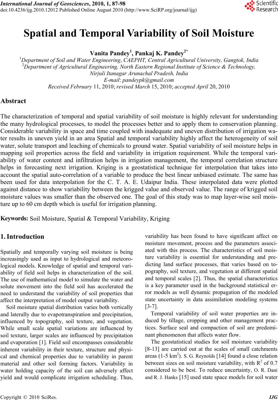 International Journal of Geosciences, 2010, 1, 87-98 doi:10.4236/ijg.2010.12012 Published Online August 2010 (http://www.SciRP.org/journal/ijg) Copyright © 2010 SciRes. IJG Spatial and Te mporal Variability of Soil Moisture Vanita Pandey1, Pankaj K. Pandey2* 1Department of So il and Water Engineering, CAEPHT, Central Agricultural University, Gangtok, India 2Department of Agricultural Engineering, North Ea stern Regional Institute of Science & Technology, Nirjuli Itanagar Arunachal Pradesh, India E-mail: pandeypk@gmail.com Received February 11, 201 0; revised Marc h 15, 2010; accepted April 20, 2010 Abstract The characterization of temporal and spatial variability of soil moisture is highly relevant for understanding the many hydrological processes, to model the processes better and to apply them to conservation planning. Considerable variability in space and time coupled with inadequate and uneven distribution of irrigation wa- ter results in uneven yield in an area Spatial and temporal variability highly affect the heterogeneity of soil water, solute transport and leaching of chemicals to ground water. Spatial variability of soil moisture helps in mapping soil properties across the field and variability in irrigation requirement. While the temporal vari- ability of water content and infiltration helps in irrigation management, the temporal correlation structure helps in forecasting next irrigation. Kriging is a geostatistical technique for interpolation that takes into account the spatial auto-correlation of a variable to produce the best linear unbiased estimate. The same has been used for data interpolation for the C. T. A. E. Udaipur India. These interpolated data were plotted against distance to show variability between the krigged value and observed value. The range of krigged soil moisture values was smaller than the observed one. The goal of this study was to map layer-wise soil mois- ture up to 60 cm depth which is useful for irrigation planning. Keywords: Soil Moisture, Spatial & Temporal Variability, Kriging 1. Introduction Spatially and temporally varying soil moisture is being increasingly used as input to hydrological and meteoro- logical models. Knowledge of spatial and temporal vari- ability of field soil helps in characterization of the soil. The use of mathematical model to simulate the water and solute movement into the field soil has accelerated the need to understand the variability of soil properties that affect the interpretation of model output variability. Soil moisture spatial distribution varies both vertically and laterally due to evapotranspiration and precipitation, influenced by topography, soil texture, and vegetation. While small scale spatial variations are influenced by soil texture, larger scales are influenced by precipitation and evaporation [1]. Field soil encompasses considerable inherent variability in their texture, structure and physi- cal and chemical properties due to variability in parent material and other soil forming factors. Variability in water holding capacity of the soil can adversely affect yield and would complicate irrigation scheduling. Thus, variability has been found to have significant affect on moisture movement, process and the parameters associ- ated with this process. The characteristics of soil mois- ture variability is essential for understanding and pre- dicting land surface processes, that varies based on to- pography, soil texture, and vegetation at different spatial and temporal scales [2]. Thus, the spatial characteristics is a key parameter used in the background statistical er- ror models as well dynamic propagation of the modeled state uncertainty in data assimilation modeling systems [3-7]. Temporal variability of soil water properties are in- duced by tillage, cropping and other management prac- tices. Surface seal and compaction of soil are predomi- nant phen omenon tha t affects wa ter flow. The geostatistical studies for soil moisture variability [8-13] are carried out at the scales of small catchments areas (1-5 km2). S. G. Reynolds [14] found a close relation between sizes on soil moisture variability, with R2 of 0.7 considered to be best. To reduce uncertainty, O. R. Dani and R. J. Hanks [15] used state space models for soil water 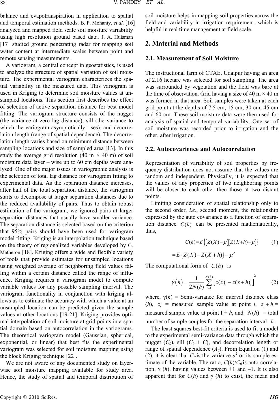 V. PANDEY ET AL. Copyright © 2010 SciRes. IJG 88 balance and evapotranspiration in application to spatial and temporal estimation methods. B. P. Mohanty, et al. [16] analyzed and mapped field scale soil moisture variability using high resolution ground based data. J. A. Huisman [17] studied ground penetrating radar for mapping soil water content at intermediate scales between point and remote sensing measurements. A variogram, a central concept in geostatistics, is used to analyze the structure of spatial variation of soil mois- ture. The experimental variogram characterizes the spa- tial variability in the measured data. This variogram is used in Kriging to determine soil moisture values at un- sampled locations. This section first describes the effect of selection of active separation distance for best model fitting. The variogram structure consists of the nugget (the variance at zero lag distance), sill (the variance to which the variogram asymptotically rises), and decorre- lation length (range of spatial dependence). The decorre- lation length varies based on minimum distance between sampling locations and size of sampled area [13]. In this study the average grid resolution (40 m × 40 m) of soil moisture data layer – wise up to 60 cm depths were ana- lysed. One of the major issues in variographic an alysis is the selection of total lag distance for variogram fitting to experimental data. As the separation distance increases, after half of the total separation distance, the variogram starts to decompose at larger separation distances due to the reduced availability of pairs. Thus to obtain robust estimation of the variogram, we ignored pairs at larger separation distances that usually have smaller variance. The separation distance is selected based on the criterion that 95% pairs should have been used for variogram model fitting. Kriging is an interpolation techniqu e based on the theory of regionalized variables developed by G. Matheron [18]. Kriging offers a wide and flexible variety of tools that provide estimates for unsampled locations using weighted average of neighboring field values fal- ling within a certain distance called the range of influ- ence. Kriging requires a variogram model to compute variable values for any possible sampling interval. The variogram functionality in conjunction with kriging al- lows us to estimate the accuracy with which a value at an unsampled location can be predicted given the sample values at other locations [19-21]. Kriging provides opti- mal interpolation of so il moisture at grid points in a sp a- tial domain based on autocorrelation in the variograms. The theoretical variogram model (Gaussian, spherical, exponential, or linear) that best fits the experimental variogram was selected for soil moisture mapping using the block Kriging technique [22]. We are not aware of any documented study on layer- wise soil moisture mapping available for study area. Hence, the study of spatial and temporal distribution of soil moisture helps in mapping soil properties across the field and variability in irrigation requirement, which is helpful in real time management at field scale. 2. Material and Methods 2.1. Measurement of Soil Moisture The instructional farm of CTAE, Udaipur having an area of 2.16 hectare was selected for soil sampling. The area was surrounded by vegetation and the field was bare at the time of observation. Grid having a si ze of 40 m × 40 m was formed in that area. Soil samples were taken at each grid point at the depths of 7.5 cm, 15 cm, 30 cm, 45 cm and 60 cm. These soil moisture data were then used for analysis of spatial and temporal variability. One set of soil moisture was recorded prior to irrigation and the other, after irrigation. 2.2. Autocovarience and Autocorrelation Representation of variability of soil properties by fre- quency distribution does not assume that the values are random and independent. Physically, it is expected that the values of any properties of two neighboring points will be closer to each other then those at two distant points. Limiting consideration of spatial relationship only to the second order, i.e., second moment, the relationship expressed by the auto covariance as a function of separa- tion distance ()Ch can be presented mathematically, thus, ()( )()ChEZXZXh (1) 2 () ()EZXZXh The computational form of ()Ch is 2 () 1 1() () 2() Nh ii i hzxzxh Nh (2) where, γ(h) = Semi-variance for interval distance class (h), i z = measured sample value at point i, i zh = measured sample value at point I + h, and ()Nh = total number of sample couples for the separation interval h. The least squares best-fit criteria is used to fit a model to the experimental semi-variance data through which the nugget (C0), sill (C0 + C), and decorrelation length or range of spatial dependence (A0). From Equation (1) and (2), it is clear that C0 is the variance σ2 or its sample es- timate of the variable. The ratio, C(h)/C0 is auto correla- tion, γ (h), having values between +1 and –1. It is also apparent that for C(h) and γ (h) to exist, the mean and 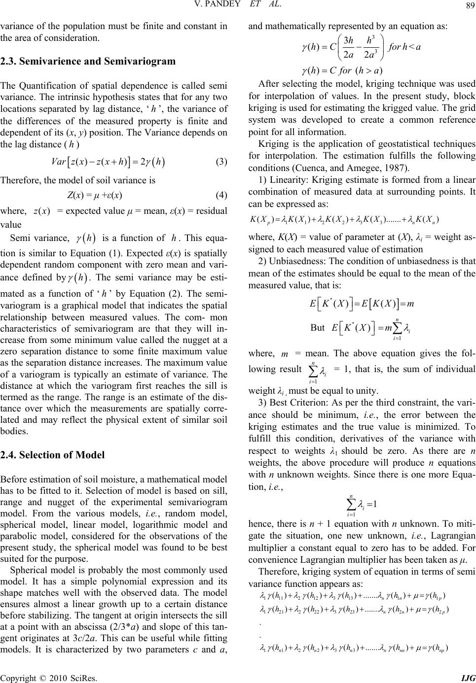 V. PANDEY ET AL. Copyright © 2010 SciRes. IJG 89 variance of the population must be finite and constant in the area of consideration. 2.3. Semivarience and Semivariogram The Quantification of spatial dependence is called semi variance. The intrinsic hypothesis states that for any two locations separated by lag distance, ‘h’, the variance of the differences of the measured property is finite and dependent of its (x, y) position. The Variance d epends on the lag distance (h) () ()2Varz xz xhh (3) Therefore, the model of soil variance is Z(x) = μ +ε(x) (4) where, ()zx = expected value μ = mean, ε(x) = residual value Semi variance, h is a function of h. This equa- tion is similar to Equation (1). Expected ε(x) is spatially dependent random component with zero mean and vari- ance defined by h . The semi variance may be esti- mated as a function of ‘h’ by Equation (2). The semi- variogram is a graphical model that indicates the spatial relationship between measured values. The com- mon characteristics of semivariogram are that they will in- crease from some minimum value called the nugget at a zero separation distance to some finite maximum value as the separation distance increases. The maximum value of a variogram is typically an estimate of variance. The distance at which the variogram first reaches the sill is termed as the range. The range is an estimate of the dis- tance over which the measurements are spatially corre- lated and may reflect the physical extent of similar soil bodies. 2.4. Selection of Model Before estimation of soil moisture, a mathematical model has to be fitted to it. Selection of model is based on sill, range and nugget of the experimental semivariogram model. From the various models, i.e., random model, spherical model, linear model, logarithmic model and parabolic model, considered for the observations of the present study, the spherical model was found to be best suited for the purpose. Spherical model is probably the most commonly used model. It has a simple polynomial expression and its shape matches well with the observed data. The model ensures almost a linear growth up to a certain distance before stabilizing. Th e tangent at origin intersects the sill at a point with an abscissa (2/3*a) and slope of this tan- gent originates at 3c/2a. This can be useful while fitting models. It is characterized by two parameters c and a, and mathematically represented by an equation as: 3 3 3 () < 22 () () hh hC forha aa hCforha After selecting the model, kriging technique was used for interpolation of values. In the present study, block kriging is used fo r estimating the krigged valu e. The grid system was developed to create a common reference point for all information. Kriging is the application of geostatistical techniques for interpolation. The estimation fulfills the following conditions (Cuenca, and Amegee, 1987). 1) Linearity: Kriging estimate is formed from a linear combination of measured data at surrounding points. It can be expressed as: 112 233 ()( )()( ).......() p nn KX KXKX KXKX where, K(X) = value of parameter at (X), λi = weight as- signed to each measured value of estimation 2) Unbiasedness: The condition of unbiasedness is that mean of the estimates should be equal to the mean of the measured value, that is: '' () ()EK XEKXm But '' 1 () n i i EK Xm where, m = mean. The above equation gives the fol- lowing result 1 n i i = 1, that is, the sum of individual weight λi , must be equal to unity. 3) Best Criterion: As per the third constraint, the vari- ance should be minimum, i.e., the error between the kriging estimates and the true value is minimized. To fulfill this condition, derivatives of the variance with respect to weights λ1 should be zero. As there are n weights, the above procedure will produce n equations with n unknown weights. Since there is one more Equa- tion, i.e., 1 1 n i i hence, there is n + 1 equation with n unknown. To miti- gate the situation, one new unknown, i.e., Lagrangian multiplier a constant equal to zero has to be added. For convenience Lagrangian multiplier has been taken as μ. Therefore, kriging system of equation in terms of semi variance function appears as: 111 21231311 121 22232322 112 233 ()( )().......( )() ()()() .......()() . . ()()() .......()() nn p nn p nnnn nnnp hhhh h hhhh h hhhh h 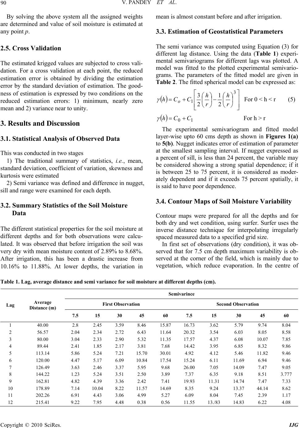 V. PANDEY ET AL. Copyright © 2010 SciRes. IJG 90 By solving the above system all the assigned weights are determined and value of soil moisture is estimated at any point p. 2.5. Cross Validation The estimated krigged values are subjected to cross vali- dation. For a cross validation at each point, the reduced estimation error is obtained by dividing the estimation error by the standard deviation of estimation. The good- ness of estimation is expressed by two conditions on the reduced estimation errors: 1) minimum, nearly zero mean and 2) variance near to unity. 3. Results and Discussion 3.1. Statistical Analysis of Observed Data This was conducted in two stages 1) The traditional summary of statistics, i.e., mean, standard deviation, coefficient of variation, skewness and kurtosis were estimated 2) Semi variance was defined and difference in nugget, sill and range were examined for each depth. 3.2. Summary Statistics of the Soil Moisture Data The different statistical properties for the soil moisture at different depths and for both observations were calcu- lated. It was observed that before irrigation the soil was very dry with mean moisture con tent of 2.89% to 8.68%. After irrigation, this has been a drastic increase from 10.16% to 11.88%. At lower depths, the variation in mean is almost constant before and after irrigation. 3.3. Estimation of Geostatistical Parameters The semi variance was computed using Equation (3) for different lag distance. Using the data (Table 1) experi- mental semivariograms for different lags was plotted. A model was fitted to the plotted experimental semivario- grams. The parameters of the fitted model are given in Table 2. The fitted spherical model can be expressed as: 3 12 1 2 3 r h r h CCh o Fo r 0 < h < r (5) 10 CCh For h > r The experimental semivariogram and fitted model layer-wise upto 60 cms depth as shown in Figures 1(a) to 5(b). Nugget indicates error of estimation of parameter at the smallest sampling interval. If nugget expressed as a percent of sill, is less than 24 percent, the variable may be considered showing a strong spatial dependence; if it is between 25 to 75 percent, it is considered as moder- ately dependent and if it exceeds 75 percent spatially, it is said to have poor dependence. 3.4. Contour Maps of Soil Moisture Variability Contour maps were prepared for all the depths and for both dry and wet condition, using surfer. Surfer uses the inverse distance technique for interpolating irregularly spaced measured data to a specified grid size. In first set of observations (dry condition), it was ob- served that for 7.5 cm depth maximum variability is ob- served at the corner of the field, which is mainly due to vegetation, which reduce evaporation. In the centre of Table 1. Lag, average distance and semi variance for soil moisture at different depths (cm). Semivarince First Observation Second Observation Lag Average Distance (m) 7.5 15 30 45 60 7.5 15 30 45 60 1 40.00 2.8 2.45 3.59 8.46 15.87 16.73 3.62 5.79 9.74 8.04 2 56.57 2.04 2.34 2.72 6.43 11.64 20.32 3.54 6.03 8.05 8.58 3 80.00 3.04 2.33 2.90 5.32 11.35 17.57 4.37 6.08 10.07 7.85 4 89.44 2.41 1.85 2.17 3.81 7.68 14.42 3.95 6.85 8.32 9.86 5 113.14 5.86 5.24 7.21 15.70 30.01 4.92 4.12 5.46 11.82 9.46 6 120.00 4.47 5.17 6.09 10.84 17.54 15.24 6.11 11.69 6.94 9.46 7 126.49 3.63 2.46 3.37 5.95 9.68 26.00 7.05 14.09 7.47 9.05 8 144.22 1.23 5.24 3.51 2.50 3.89 7.37 6.35 9.18 8.51 3.777 9 162.81 4.82 4.39 3.36 2.42 7.41 19.93 11.31 14.74 7.47 7.33 10 178.89 7.14 10.04 8.22 11.57 14.69 8.35 9.24 13.37 44.14 8.62 11 202.26 6.91 4.43 3.06 4.99 5.27 6.09 8.04 7.45 2.39 1.17 12 215.41 9.22 7.95 4.48 0.38 0.56 11.55 13./83 14.83 6.22 4.08  V. PANDEY ET AL. Copyright © 2010 SciRes. IJG 91 Table 2. Different parameters of the fitted model of semivariogram. S.No Depth (cm) Type of Model Range Nugget Sill Nugget as % of Sill Spatial Dependence First Observation 1 7.5 Spherical 125 0.45 3.05 14.75 Strongly dependent 2 15 Spherical 113.1 0.327 2.947 11.09 Strongly dependent 3 30 Spherical 110 0.46 3.1 14.84 Strongly dependent 4 45 Spherical 113.09 0.638 5.748 11.09 Strongly dependent 5 60 Spherical 113.09 1.1787 10.61 11.10 Strongly dependent Second Observation 1 7.5 Spherical 125 2.1 14 15 Strongly dependent 2 15 Spherical 113.09 0.548 4.94 11.09 Strongly dependent 3 30 Spherical 113.09 0.836 7.525 11.10 Strongly dependent 4 45 Spherical 113.09 0.848 7.634 11.10 Strongly dependent 5 60 Spherical 113.09 0.804 7.244 11.09 Strongly dependent the field, soil moisture is almost constant Figure 6(a), which is due to the bare field, which provides a free evaporation surface. As shown in Figure 7(a) for 15 cm depth, variability is large as compared to 7.5 cm depth, but the same pat- tern is observed at this depth, i.e., maximum in the cor- ners and minimum at the centre. Mean moisture content at 15 cm depth is higher than 7.5 cm depth. As shown in Figures 8(a), Figure 9(a) and Figure 10 (a) shows a uniform spatial variability with 30 cm depth, 45 cm depth and 60 cm depth respectively. Mean mois- ture content was found higher at 60 cm depth than other depths. In the second set of observations, it was observed that for 7.5 cm depth, moisture content at the corner of the fields is almost constant whereas in the middle it is very high which shows non uniform supp ly of water as shown in Figure 6(c). For 15 cm depth, high spatial variability is obtained as compared to 7.5 cm depth Figure 6(c). In the middle, the moisture content is very high at 7.5 cm depth due to the same reason of non uniform supply of water as shown in Figure 7(c). For 30 cm depth, 45 cm depth and 60 cm depth the variability is almost same Figure 8(c), 9(c) and 10(c), respectively. From the maps, it was observed that in the first set of observation high spatial variability was observed as com- pared to th e second set of obse rvation. This is because of the reason that the second sets of observation were taken after irrigation. Soil profile is almost saturated with water. Some variability was observed, which shows the non uniform supply of irrigation water. The maximum vari- ability is observed up to 30 cm depth where as for 45 cm and 60 cm depths, variability is almost constant in both sets of observations. In both sets of observations maxi- mum spatial variability was observed at 30 cm depth (Figures 8 (a) and 8(c)). 0 1 2 3 4 5 6 7 8 9 10 050100150 200250 Average distance (m) S emivar ian ce(%) 3 31 ( )0.453.050 21252 125 ( )0.453.05 hh hforhr hforhr (a) 0 5 10 15 20 25 30 050100 150200 250 Average distance (m) Semivariance 3 31 () 2.1140 2 1252125 () 2.114 hh hforhr hforhr (b) Figure 1. (a) Experimental semivariogram of first observa- tion at 7.5 cm depth and fitted model; (b) Experimental semivariogram of second observation at 7.5 cm depth and fitted model.  V. PANDEY ET AL. Copyright © 2010 SciRes. IJG 92 0 2 4 6 8 10 12 050100 150 200250 Average distance (m) semivar i an ce (% ) 3 31 ( )0.332.9470 2113.12 113.1 ( )0.332.947 hh hforhr hforhr 0 2 4 6 8 10 12 14 16 050100150 200 250 Average distance (m) Semivarian ce (% ) 3 31 ( )0.5494.940 2 113.092113.09 ( )0.5494.94 hh hforhr hforhr (a) (b) Figure 2. (a) Experimental semivariogram of first observation at 15 cm depth and fitted model; (b) Experimental semiva- riogram of second observation at 15 cm depth and fitted model. 0 2 4 6 8 10 12 14 16 050100150 200 250 Average distance(m) Semivariance (%) 3 31 ( )0.463.10 2110 2110 ( )0.463.1 hh hforhr hforhr 0 2 4 6 8 10 12 14 16 050100 150200 250 Average distance(m) S emivari a n ce (%) 3 31 ( )0.8367.5250 2113.092 113.09 ( )0.8367.525 hh hforhr hforhr (a) (b) Figure 3. (a) Experimental semivariogram of first observation at 30 cm depth and fitted model; (b) Experimental semiva- riogram of second observation at 30 cm depth and fitted model. 0 2 4 6 8 10 12 14 16 050100150 200 250 Average distance (m) Semivariance (%) 3 31 ( )0.6385.7480 2113.092 113.09 ( )0.6385.748 hh hforhr hforhr 0 2 4 6 8 10 12 14 16 050100 150 200 250 Average distance (m) Semivariance(%) 3 31 ( )0.8487.6340 2 113.092113.09 ( )0.8487.634 hh hforhr hforhr (a) (b) Figure 4. (a) Experimental semivariogram of first observation at 45 cm depth and fitted model; (b) Experimental semiva- riogram of second observation at 45 cm depth and fitted model.  V. PANDEY ET AL. Copyright © 2010 SciRes. IJG 93 0 4 8 12 16 20 24 28 32 36 050100 150 200250 Average distan ce (m) Semivariance (%) 3 31 ( )1.17910.610 2113.092 113.09 ( )1.17910.61 hh hforhr hforhr 0 2 4 6 8 10 12 14 16 050100150 200 250 Average distance (m) Semivarience (%) 3 31 ( )0.817.240 2 113.092 113.09 ( )0.817.24 hh hforhr hforhr (a) (b) Figure 5. (a) Experimental semivariogram of first observation at 60 cm depth and fitted model; (b) Experimental semiva- riogram of second observation at 60 cm depth and fitted model. Table 3. Statistical parameters of measured and krigged values of soil moisture. Depth Observation Max. (%) Min (%) Range (%) Mean (%) Var. S.D (%) C.V First observat i on Measured 7.89 0.92 6.97 2.93 3.50 1.87 0.64 Krigged 5.29 1.12 4.17 2.87 1.55 1.25 0.43 7.5 Second observation Measured 18.98 7.16 11.82 10.54 8.11 2.85 0.27 Krigged 14.55 5.89 8.66 10.48 5.90 2.43 0.23 First observat i on Measured 7.67 1.44 6.23 4.07 3.27 1.81 0.44 Krigged 6.16 2.30 3.86 4.05 1.64 1.28 0.32 15 Second observation Measured 15.12 7.26 7.86 10.16 4.90 2.21 0.22 Krigged 13.53 7.70 5.83 10.15 2.91 1.71 0.17 First observat i on Measured 9.30 2.63 6.67 5.38 3.56 1.89 0.35 Krigged 7.68 3.33 4.35 5.33 1.91 1.38 0.26 30 Second observation Measured 12.84 6.61 6.23 10.21 4.68 2.16 0.21 First observat i on Measured 12.36 3.28 9.08 7.20 6.39 2.53 0.35 Krigged 11.29 4.37 6.92 7.22 3.60 1.90 0.26 45 Second observation Measured 16.10 7.45 8.65 11.70 7.63 2.76 0.24 Krigged 14.36 8.59 5.77 11.64 3.33 1.82 0.16 First observat i on Measured 14.60 3.25 11.35 8.68 11.8 3.43 0.40 Krigged 12.97 5.12 7.85 8.81 6.73 2.59 0.29 60 Second observation Measured 16.63 7.60 10.30 11.88 5.60 2.37 0.20 Krigged 14.70 9.01 5.69 11.91 3.35 1.83 0.15  V. PANDEY ET AL. Copyright © 2010 SciRes. IJG 94 3.5. Kriging of Soil Moisture In order to estimate the soil moisture value at observation point, the searching radius was determined, which was based on spatial range observed in the fitted model of semivariogram. The searching radius indicates that the measurements within the range are to be considered to estimate the soil moisture at that point. Range for each depth as shown in Table 2. By using Sill, range and nugget as shown in Table 1, the krigged value of soil moisture were determined at each depth with the help of Datamine software. Statisti- cal parameters were calculated for measured and krigged soil moisture values and the parameters are presented in Table 3. Mean and measured krigged value is almost same. By analyzing the statistical parameters, i.e., vari- ance, standard deviation and coefficient of variation, it was found that they have always been on the lower side of the krigged estimate as compared to those obtained with measured value, the trend is indicative of lesser variability in the krigged estimates of soil moisture there- by projecting more consistency and reliability. The lower value of coefficient of variation of krigged value indi- cates that there has been consistency in krigged estimates. 3.6. Comparison of Spatial Structure of Measured and Krigged Soil Moisture Contour maps of soil moisture variability were plotted for measurement and krigged values for each depth and for both observations and their variability and spatial structure were compared (Figures 6(b), 6(d), 7(b), 7(d), 8(b), and 8(d), 9(b), 9(d), 10(b), 10(d)). Large variabil- ity is observed in first observation, i.e., before irrigation compared to second observation, which is spatially less variable. For first observation large variability is observed (a) (b) (c) (d) Figure 6. (a) and (b) measured and krigged value of soil moisture at 7.5 cm depth for dry condition, (c) and (d) measured and krigged value of soil moisture at 7.5 cm depth for wet condition.  V. PANDEY ET AL. Copyright © 2010 SciRes. IJG 95 (a) (b) (c) (d) Figure 7. (a) and (b) measured and krigged value of soil moisture at 15 cm depth for dry condition; (c) and (d) measured and krigged value of soil moisture at 15 cm depth for wet condition. (a) (b)  V. PANDEY ET AL. Copyright © 2010 SciRes. IJG 96 (c) (d) Figure 8. (a) and (b) measured and krigged value of soil moisture at 30 cm depth for dry condition; (c) and (d) measured and krigged value of so il moisture at 30 cm depth for wet condition. (a) (b) (c) (d) Figure 9. (a) and (b) measured and krigged value of soil moisture at 45 cm depth for dry condition; (c) and (d) measured and krigged value of so il moisture at 45 cm depth for wet condition.  V. PANDEY ET AL. Copyright © 2010 SciRes. IJG 97 (a) (b) (c) (d) Figure 10. (a) and (b) measured and krigged value of soil moisture at 60 cm depth for dry condition; (c) and (d) measured and krigged value of so il moisture at 60 cm depth for wet condition. at 30 cm depth as in Figure 8(a) and comparatively less variability is observed at 7.5 cm depth as in Figure 6(a) due to lack of moisture. After kriging, the variability was reduced as shown in krigged map. Also the range of the krigged values are less than that of the observed one (Table 3). For second observation the largest variability was ob- served at 15 cm depth as in Figure 7(c), which was re- duced drastically for krigged estimate whereas least variability was observed at 7.5 cm depth. The range of second observation indicates that the water is not uni- formly distributed in the whole field. For the lower depths, the variability is almost same for both sets of observations for measured as well as krigged estimates, because some time is required for water to percolate down and during that time sufficient variability is ob- served at lower depth. From the maps, it was observed that the spatial vari- ability is considerably reduced after kriging for each depth, especially for second observation. Contour maps of soil moisture for each depth were plotted. Careful comparison of the contour map of soil moisture envisaged that there has been considerable re- duction in spatial variability in case of krigged estimates. On the basis of the above discussion, it can be said that the krigged values are more consistent and are true rep- resentative of soil moisture values. Therefore, contour maps developed with krigged estimates would be more precise than those developed with measured value. 4. Conclusions Based on the findings it can be said that the krigged val-  V. PANDEY ET AL. Copyright © 2010 SciRes. IJG 98 ues are more consistent and true representative of soil moisture values. Hence, on the basis of past soil moisture values the krigged value of soil moisture at particular time and space may be estimated. Statistical parameters reflect that the variability of soil moisture reduces sig- nificantly after kriging. These estimated values help in proper irrigation scheduling along with necessary infor- mation on the crops to be grown and expected yield of the same. 5. References [1] A. Oldak, T. Jackson and Y. Pachepsky, “Using GIS in Passive Microwave Soil Mapping and Geostatistical Analysis,” International Journal of Geographical Infor- mation Science, Vol. 16, No. 7, 2002, pp. 681-689. [2] A. J. Teuling and P. A. Troch, “Improved Understanding of Soil Moisture Variability Dynamics,” Geophysical Research Letters, Vol. 32, No. 5, 2005, p. 4 [3] M. Durand and S. Margulis, “Effects of Uncertainty Magnitude and Accuracy on Assimilation of Multi-Scale Mea- surements for Snowpack Characterization,” Journal of Ge- ophysical Research, Vol. 113, No. 16, 2008, p. 17. [4] M. Zupanski, D. Zupanski, D. F. Parrish, E. Rogers and G. DiMego, “Four-Dimensional Variation Data Assimila- tion for the Blizzard of 2000,” Monthly Weather Review, Vol. 130, No. 8, 2002, pp. 1967-1988. [5] T. Vukicevic, M. Sengupta, A. S. Jones and T. Von- der-Haar, “Cloud-Resolving Satellite Data Assimilation: Information Content of IR Window Observations and Uncertainties in Estimation,” Journal of the Atmospheric Sciences, Vol. 63, No. 3, 2006, pp. 901-919. [6] W. T. Crow, “Correcting Land Surface Model Predictions for the Impact of Temporally Sparse Rainfall Rate Meas- urements Using an Ensemble Kalman Filter and Surface Brightness Temperature Observations,” Journal of Hy- dro- meteorology, Vol. 4, No. 5, 2003, pp. 960-973. [7] M. Zupanski, S. J. Fletcher, I. M. Navon, B. Uzunoglu, R. P. Heikes, D. A. Ra ndall, T. D. Ringler a nd D. N. Daescu, “Initiation of Ensemble Data Assimilation,” Tellus A, Vol. 58, No. 2, 2006, pp. 159-170. [8] F. Anctil, R. Mathieu, L.-E. Parent, A. A. Viau, M. Sbih, and M. Hessami, “Geostatistics of Near-Surface Moisture in Bare Cultivated Organic Soils,” Journal of Hydrology, Vol. 260, No. 1, 2002, pp. 30-37. [9] A. Bardossy and W. Lehmann, “Spatial Distribution of Soil Moisture in a Small Catchment. Part 1: Geostatistical Analysis,” Journal of Hydrology, Vol. 206, No. 1, 1998, pp. 1-15. [10] M. Herbst and B. Diekkruger, “Modelling the Spatial Variability of Soil Moisture in a Micro-Scale Catchment and Comparison with Field Data Using Geostatistics,” Physics and Chemistry of the Earth, Parts A/B/C, Vol. 28, No. 6, 2003, pp. 239-245. [11] J. Wang, B. Fu, Y. Qiu, L. Chen and Z. Wang, “Geosta- tistical Analysis of Soil Moisture Variability on Da Nan- gou Catchment of the Loess Plateau, China,” Environ- mental Geology, Vol. 41, No. 1-2, 2001, pp. 113-120. [12] A. W. Western, R. B. Grayson and T. R. Green, “The Tarrawarra Project: High Resolution Spatial Measure- ment, Modelling and Analysis of Hydrological Re- sponse,” Hydrological Processes, Vol. 13, No. 5, 1999, pp. 633-652. [13] A. W. Western, G. Blöschl and R. B. Grayson, “Geosta- tistical Characterization of Soil Moisture Patterns in the Tarrawarra a Catchment,” Journal of Hydrology, Vol. 217, No. 3, 1999, pp. 203-224. [14] S. G. Reynolds, “A Note on Relationship between the Size of Area and Soil Moisture Variability,” Journal of Hydrology, Vol. 22, 1974, pp. 71-76. [15] O. R. Dani and R. J. Hanks, “Spatial and Temporal Soil Moisture Estimation Considering Soil Variability and Evapotranspiration on Uncertainty,” Water Resources Research, Vol. 28, No. 3, 1992, pp. 803-814. [16] B. P. Mohanty, T. H. Skaggs and J. S. Famiglietti, “Analysis and Mapping of Field Scale Soil Moisture Variability Using High Resolution Ground Based Data during the Southern Great Plains,” Water Resources Re- search, Vol. 36, No. 4, 2000, pp. 1023-1031. [17] J. A. Huisman, C. Sperl, W. Bouten and J. M. Verstraten, “Soil Water Content Measurent at Different Scales: Ac- curacy of Time Domain Reflectometery and Ground Penetrating Radar,” Journal of Hydrology, Vol. 245, No. 1, 2001, pp. 48-58. [18] G. Matheron, “La the´ orie des Variables re´ Gionalise´ es et ses Applications,” Masson et Cie, Paris, 1965. [19] E. H. Isaaks and R. M. Srivastava, “Applied Geostatis- tics,” Oxford University Press, New York, 1989. [20] R. E. Rossi, J. L. Dungan and L. R. Beck, “Kriging in the Shadows: Geostatistical Interpolation for Remote Sens- ing,” Remote Sensing of Environment, Vol. 49, No. 1, 1994, pp. 32-40. [21] A. U. Bhatti, D. J. Mulla and B. E. Frazier, “Estimation of Soil Properties and Wheat Yields on Complex Eroded Hills Using Geostatistics and Thematic Mapper Images,” Remote Sensing of Environment, Vol. 37, No. 3, 1991, pp. 181-191. [22] R. Webster and M. A. Oliver, “Geostatistics for Envi- ronmental Scientists,” John Wiley & Sons Ltd, Chiches- ter, 2001. |