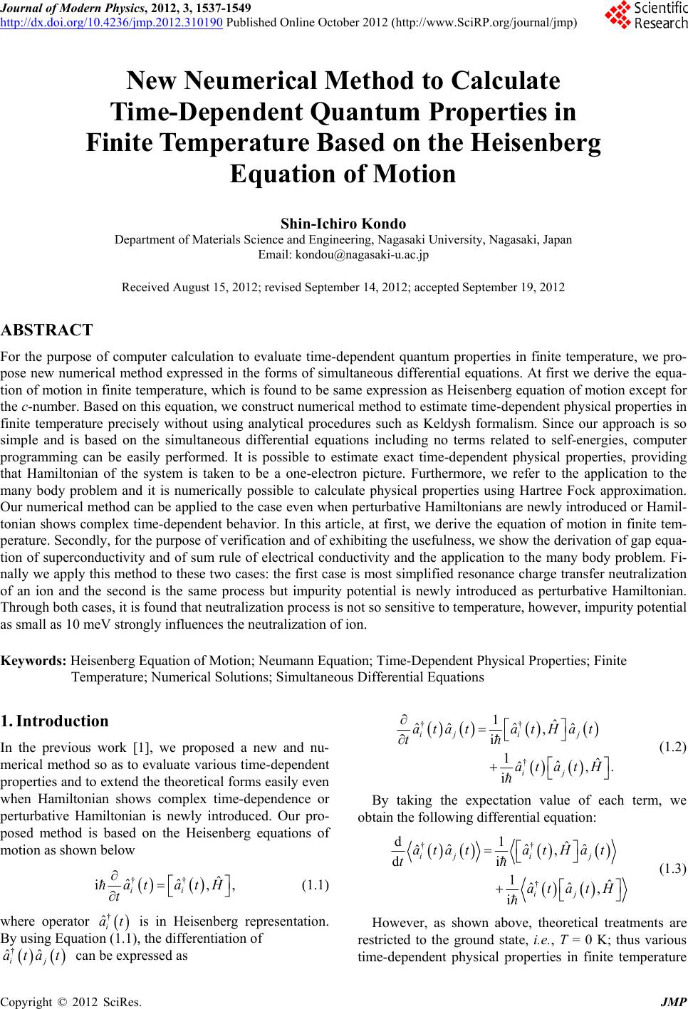
 Journal of Modern Physics, 2012, 3, 1537-1549 http://dx.doi.org/10.4236/jmp.2012.310190 Published Online October 2012 (http://www.SciRP.org/journal/jmp) New Neumerical Method to Calculate Time-Dependent Quantum Properties in Finite Temperature Based on the Heisenberg Equation of Motion Shin-Ichiro Kondo Department of Materials Science and Engineering, Nagasaki University, Nagasaki, Japan Email: kondou@nagasaki-u.ac.jp Received August 15, 2012; revised September 14, 2012; accepted September 19, 2012 ABSTRACT For the purpose of computer calculation to evaluate time-dependent quantum properties in finite temperature, we pro- pose new numerical method expressed in the forms of simultaneous differential equations. At first we derive the equa- tion of motion in finite temperature, which is found to be same expression as Heisenberg equation of motion except for the c-number. Based on this equation, we construct numerical method to estimate time-dependent physical properties in finite temperature precisely without using analytical procedures such as Keldysh formalism. Since our approach is so simple and is based on the simultaneous differential equations including no terms related to self-energies, computer programming can be easily performed. It is possible to estimate exact time-dependent physical properties, providing that Hamiltonian of the system is taken to be a one-electron picture. Furthermore, we refer to the application to the many body problem and it is numerically possible to calculate physical properties using Hartree Fock approximation. Our numerical method can be applied to the case even when perturbative Hamiltonians are newly introduced or Hamil- tonian shows complex time-dependent behavior. In this article, at first, we derive the equation of motion in finite tem- perature. Secondly, for the purpose of verification and of exhibiting the usefulness, we show the derivation of gap equa- tion of superconductivity and of sum rule of electrical conductivity and the application to the many body problem. Fi- nally we apply this method to these two cases: the first case is most simplified resonance charge transfer neutralization of an ion and the second is the same process but impurity potential is newly introduced as perturbative Hamiltonian. Through both cases, it is found that neutralization process is not so sensitive to temperature, however, impurity potential as small as 10 meV strongly influences the neutralization of ion. Keywords: Heisenberg Equation of Motion; Neumann Equation; Time-Dependent Physical Properties; Finite Temperature; Numerical Solutions; Simultaneous Differential Equations 1. Introduction In the previous work [1], we proposed a new and nu- merical method so as to evaluate various time-dependent properties and to extend the theoretical forms easily even when Hamiltonian shows complex time-dependence or perturbative Hamiltonian is newly introduced. Our pro- posed method is based on the Heisenberg equations of motion as shown below † ˆ iat t †ˆ ˆ,, ii atH † ˆ at (1.1) where operator i is in Heisenberg representation. By using Equation (1.1), the differentiation of can be expressed as † ˆˆ i ata j t †† † 1ˆ ˆˆˆˆ , i 1ˆ ˆˆ,. i iji j ij atat atHat t atatH (1.2) By taking the expectation value of each term, we obtain the following differential equation: †† † d1 ˆ ˆˆˆˆ , di 1ˆ ˆˆ, i iji j ij atat atHat t atatH (1.3) However, as shown above, theoretical treatments are restricted to the ground state, i.e., T = 0 K; thus various time-dependent physical properties in finite temperature C opyright © 2012 SciRes. JMP 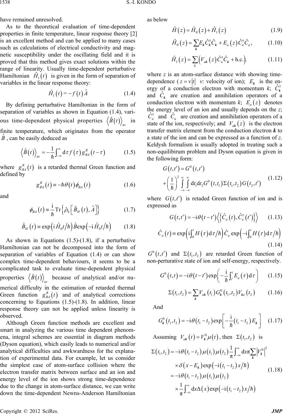 S.-I. KONDO 1538 have remained unresolved. As to the theoretical evaluation of time-dependent properties in finite temperature, linear response theory [2] is an excellent method and can be applied to many cases such as calculations of electrical conductivity and mag- netic susceptibility under the oscillating field and it is proved that this method gives exact solutions within the range of linearity. Usually time-dependent perturbative Hamiltonian 1 ˆ t ˆ = is given in the form of separation of variables in the linear response theory: 1 ˆ tftA (1.4) By defining perturbative Hamiltonian in the form of separation of variables as shown in Equation (1.4), vari- ous time-dependent physical properties av ˆ Bt ˆ B in finite temperature, which originates from the operator , can be easily deduced as R BA g t av 1 ˆdBt f R (1.5) where BA t BA is a retarded thermal Green function and defined by R BA t tt (1.6) and ˆ ˆ, H BtA 0 iˆ Tr BA t (1.7) 0 ˆ expi Ht 0 ˆˆ ˆ exp i H BtHtB (1.8) As shown in Equations (1.5)-(1.8), if a perturbative Hamiltonian can not be decomposed into the form of separation of variables of Equation (1.4) or can show complex time-dependent behaviours, it seems to be a complicated task to evaluate time-dependent physical properties av ˆ Bt R because of analytical and/or nu- merical difficulty in the estimation of retarded thermal Green function BA t and of analytical corrections concerning to Equations (1.5)-(1.8). In addition, linear response theory can not be applied unless linearity is observed. Although Green function methods are excellent and smart in analyzing the various time dependent phenom- ena, integral schemes are essential in diagram methods (Dyson equation), which easily leads to numerical and/or analytical difficulties and awkwardness for the explana- tion of experimental data. For example, let us consider the simplest case of atom-surface collision where the electron transfer matrix between surface and an ion and energy level of the ion shows strong time-dependence due to the change in atom-surface distance, we can write down the time-dependent Newns-Anderson Hamiltonian as below 01 ˆˆ ˆ zHzHz (1.9) †† 0ˆˆ ˆˆ ˆ, aaa zECCEzCC (1.10) kkk k † 1ˆˆ ˆh.c. . aa k HzV zCC kk (1.11) where z is an atom-surface distance with showing time- dependence (zvtE † ˆ C ˆ C Ez † ˆ Cˆ Vz v: velocity of ion); k is the en- ergy of a conduction electron with momentum k; k and k are creation and annihilation operators of a conduction electron with momentum k; a denotes the energy level of an ion and usually depends on the z; a and a C are creation and annihilation operators of a state of the ion, respectively; and ak is the electron transfer matrix element from the conduction electron k to a state of the ion and can be expressed as a function of z. Keldysh formalism is usually adopted in treating such a non-equilibirum problem and Dyson equation is given in the following form: 0 2 0 121 122 ,, 1dd ,,, GttGtt ttGtttt Gtt (1.12) ,Gtt where is retaded Green function of ion and is expressed as † ˆˆ ,i , aa GttttC t Ct (1.13) 00 ˆˆ exp idexpid tt aa CtH C H (1.14) 0,Gtt and ,tt 12 are retarded Green function of non-perturative state of ion and self-energy, respectively. 0i ,i expd t a t Gtt ttE (1.15) 0 121 122 ,, aa ttVt GttVt kk k k (1.16) And 0 12 1212 i ,i expGttttt tE kk (1.17) Assuming 0 a Vt Vt kk 12 ,tt , then is 2 0 121212 12 12 1 2 12 1 ,i dπ π exp i i 1dΔexp i π ttt tttxV xEttx tttt xx ttx k k k (1.18) Copyright © 2012 SciRes. JMP  S.-I. KONDO 1539 where 2 0 π VxE kk n k (1.19) The number of electron on the ion at t, i.e. , , which we should seek and calculate, is 22 ,,G kk ,Gtt k nnG n k (1.20) In above equation, nkdenotes the number of electron occupying the band state k at initial state and is given 0 11 ,, V Gtt Gtt k k 0 1 1 ,dtGtt t k n n (1.21) As shown in the series of Equations (1.12) to (1.21), many calculations and procedures are necessary to evalu- ate , which suggest that analytical efforts to evalu- ate are usually failed except for a few cases. Since energy state of ion Et 0,Gtt 0,Gtt a, which is experiment- tally determined, is considered complex, we can easily guess analytical form of can not be obtainable and numerical expression of is only possible. Additionally analytical procedures to treat the term 0 VV in Equation (1.19) is very difficult except for a few cases. Usually the assumption of k (k independence) is strongly required, thus Equation (1.19) is 0 22 00 2 0 ππ π VxE V Vx kk k xE k k (1.22) In the above equation, E 00 VV is D.O.S (Density of States) for conduction electrons. The assumption of k (k independence) is a very rough approxima- tion and actual the systems seem to have k dependence, thus this approximation may not match the analysis of experimental data. Next, let us discuss the term of self energy . By substituting Equation (1.22) into Equation (1.18), we obtain following expression for self energy: 12 ,tt 2 0 2 12 i t V ttx ,tt 12 1 21 ,i dexp ttt tt xx (1.23) Usually the term of 12 of Equation (1.23) can not be evaluated in the analytical form except for the specific cases such as or E 0cons t E 00 , therefore, the procedure on the basis of (1.12) seems too complicated even if perturbative method is used. Consequently awkward and complex analytical and/or numerical schems for calculating integral parts and a lot of approximations ignoring experimental condi- tions are essentially required to evaluate . Actually, theoretical solutions are obatined in the limited condi- tions such as wide band limit. n ˆ EE Furthermore, if there exists impurity atoms or disloca- tions on surface, we should take account of the presence of impurity potential as shown below † ˆˆ ˆ.VCC (1.24) kk' k k kk' When such a perturbative Hamiltonian is intoroduced into the system, it should be noted that the methods on the basis of Keldysh formalism seems almost impossible for evaluating n precisely because of a lots of awkward analytical and/or numerical tasks and approxi- mations ignoring experimental conditions. Concerning the other approaches, we can mention the works performed by Brako and Newns, [3,4]. Starting from the equation of motion method proposed by Bloss and Hone [5], they performed calculations by solving the simultaneous differential equations while regarding op- erators (Q-number) as c-number. Based on these ap- proaches, their method are expressed in the integral forms and exact solutions can be attainable in the case of wide band limit with assuming . Actu- ally experimental data on the polarisation of the light emitted in the electronic transition of H atoms scattered on Ni(111) surface [6] were theoretically interpreted and examined by their method [7]. Δconst an tx However, their method also seems to meet the nu- merical and analytical difficulties and nuisances when perturbative Hamiltonian is introduced or the system shows complicated time-dependence because of integral schemes being involved. Actually, their method can not be applied to the case when impurity potential as shown in Equation (1.24) is introduced into the system. Concerning these theoretical methods as stated above, the main reason for complicating calculations is that theoretical expressions are given not in the differential forms but in the integral ones. In this article, therefore, for the purpose of constructing the method which can be applicable to experimental analysis, we propose a new numerical methods on the basis of differential forms. At first we derive the extension of Heisenberg equation of motion to finite temperature. Then, based on the such an extension, we construct simultaneous differential equa- tions which can evaluate time-dependent physical prop- av ˆ Bt erties in finite temperature. Our method can be applied to the case when a perturbative Hamiltonian can show so complex time-dependent behaviours that analysis on the basis of linear response theory and/or of Green function methods seem to meet analytical difficul- ties and nuisance and even when perturbative Hamilto- nian is newly introduced. Copyright © 2012 SciRes. JMP  S.-I. KONDO 1540 In Section 2, we show the derivation of theoretical formalism and verify our proposed method for two cases: superconductivity and electrical conductivity. Further- more we refer to the application to the many body prob- lem using Hatree Fock approximation. After confirming our calculations, in Section 3, we apply our method to the two cases of resonant charge transfer processes, in which time-dependent properties play important roles on deciding dynamics. The first case is the most simlified resonant charge transfer process that a single charged ion is neutralzed in front of metal. During calculating, to simplify the discussion we assume electron transfer ma- trix remains constant. However it is sufficiently possible to estimate physical properties under the condition that electron transfer matrix shows k dependence. In the sec- ond case, we numerically treat the same process when impurity potential is introduced as perturbative Hamilto- nian. The second case is more complicated than the first one and is usually considered as a difficult and awkward task to analyze on the basis of conventional ways such as Keldysh formalism because perturbative Hamiltonian often complicates the scheme of the evaluation of self energy. Furthermore, temperature dependence of reso- nant charge transfer process under the presence of impu- rity potential remains unresolved. Finally, in Section 4 we conclude this paper and discuss the remaining prob- lems and further developments. 2. Theoretical Approach, Its Verifications and Application to Many Body Problem 2.1. Derivation of Theoretical Framework Firstly, let us start from the Neumann equation, which is given by i t ˆ ˆˆ ,,tHt (2.1) where operator ˆt is a time-dependent density op- erator. Additionally we set 0 (chemical potential) = 0 hereafter for simplifying the discussion. Then time-de- pendent physical properties av ˆ Bt in finite tempera- ture is given by ˆˆ ˆ Tr tB av Bt . (2.2) By taking the the differentiation of the above equation, we obtain ˆˆ ˆ rtB t av dd ˆˆ Tr T dd Bt tB tt (2.3) Substituting the Neumann equation of Equation (2.1) into the above equation, we get ˆˆ ,Ht B av d1 ˆTr di Bt t ˆˆˆˆ Tr Tr . (2.4) Finally, using the relation YYX , we obtain the following formula with respect to the the dif- ferential form of av ˆ Bt av av d1 ˆˆˆ ˆ Tr , di 1ˆˆ , i Btt BH t BH t (2.5) It should be easily noticed that Equation (2.5) takes the same form as Heisenberg equation of motion in Equation (1.1) except for the c-number. The above equation cor- responds to the extension of Heisenberg equation of mo- tion to finite temperature. Equation (2.5) directly leads to the fact that time-dependent physical properties av ˆ Bt 0 ††† ˆˆ ˆ = ˆˆˆˆˆˆ , KH N CCVtCCCC kk kkkkkk k kk,k 0 E in finite temperature are expressed not in the integral forms as Dyson equations but in the differential forms (simultaneous differetial equations); this, therefore, indi- cates analytical and/or numerical nuisances will be ex- pected to greatly decrease even if Hamiltonian includes complex terms and/or perturbative Hamiltonian is intro- duced. 2.2. Derivation of Gap Equation in Superconductivity Next, in order to verify the above theoretical results, let us apply the above equation to the superconductivity. we consider the following Hamiltonian: (2.6) where (2.7) kk and .VttV kk kk E † ˆ C (2.8) In the above equations, k is the energy of a con- duction electron with momentum k. k and ˆ C k are creation and annihilation operators of a conduction elec- tron with momentum k and spin orientations . Con- cerning t , this function increases monotonically and satisfies 0and 1 . (2.9) Furthermore we introduce gap function Δ,tk as defined below av ˆˆ ,.tVtCCt kq qq q k (2.10) Using mean field approximation and Equation (2.10), Copyright © 2012 SciRes. JMP  S.-I. KONDO 1541 Hamiltonian Equation (2.6) can be reduced to one- electron picture and given by † †† * †† av ˆˆ ˆ ˆˆ , ˆˆ ,. KCC tC C tC Ct kk k kσ kk k kk k k k ˆˆ , tC C k k k ˆ B ˆˆ ˆ BCC (2.11) Next, we take operator as qq ˆˆ ,BK †† ˆ ˆ ˆˆ ,. C C C qq q q (2.12) Accordingly, is ˆˆ ˆˆ , ˆˆ BKC CC tCC qq qq qq q (2.13) Then, based on the Equation (2.5), the differential form of av ˆ Bt is av av †† av dˆˆ d 1ˆˆ ˆ i ˆˆ ˆ CC t t CC tC tCCt C qq q qq qq q q av av ˆ ˆ ,. C t C t q qq q t (2.14) In the limit of , dˆˆ dCCt t t qq qq av 0 ,1 (2.15) Consequently from Equation (2.14) ˆˆ 2 1 CC qqq q av nn qq (2.16) where † † ˆ ˆ nC nC qq av av ˆ ˆ C C q qqq (2.17) By combining the above relation with Equation (2.10), we obtain 1 2 V kq qq kq nn qq t † † ˆˆ, ˆˆ, v v kk kk k kk kk k ukvk (2.18) Next, using Bogoliubov transformation to the Hamil- tonian of Equation (2.11) in the limit of ˆ ˆ Cu Cu (2.19) where and satisfies 2 21uv . (2.20) kk Then Hamiltonian can be easily diagonalized and is given by †† 2 †† av. ˆˆˆˆˆ 22 ˆˆ k KE vuv CC kk kk k kkkk k kk k k k (2.21) where 2 2 E kk k . From Bogoliubov transformation of Equation (2.19), av av 2 2 av av ˆˆ ˆˆ = ˆˆˆˆ 1 nCC CC uv qqq qq qq qqq q †† †† (2.22) av av 2 2 av av ˆˆ ˆˆ ˆˆˆˆ 1 nCC CC uv qqq qq qq qq qq †† †† (2.23) Since Hamiltonian is diagonalized as shown in Equa- tion (2.21), we can easily estimate † av ˆˆ qq and † av ˆˆ qq. Then av av ˆˆˆˆel qqqq E q †† , (2.24) el where x is a Fermi-Dirac function 11 exp el fx x . Consequently, the term of 1nn qq is 1 1tanh. 2 nn E E q q qq q (2.25) By substituting the above result into Equation (2.18), we finally obtain gap equation. 1 tanh . 22 VE E kq q qq kq (2.26) 2.3. Calculation of Electrical Conductivity Next, we apply the Equation (2.5) to the electrical con- duction. At first, we assume the following Hamiltonian: 01 2 012 =1 1 =1 ˆˆ ˆ 1 ˆˆ,,, 2 ˆ Nj jN jj N jj j HH H Q HV mc HftQ PAr rrr rE (2.27) Copyright © 2012 SciRes. JMP  S.-I. KONDO 1542 where m and Q ,, are jth mass and charge of particles respectively, c is a light velocity, and 12 V rr r is a potential term. Magnetic Field r is expressed by using vector potential Ar , i.e., rot j rAr. Electric field , vector of location r and ˆ P are 123 123 123 ,, , , ,, i , jjj j j jj j EEE x xx x 1, 2,3 123 ,, ,, ˆˆ ˆˆ ,, i, xyz jjjj jjj EEE xyz PPP xx E r P (2.28) We obtain j , the time differential form of , from the relation x j x 0 ˆˆ ,, j j j HxH Q mc Ar 3 ,, jj Ar r ˆ B i, 1ˆ jj jj j xx xP (2.29) where 12jj AAAr r. Since we focus on the electrical conduction, we take operator as an electric current density along di- rection, 1 1, Ω N kk k Qx ˆˆ Bj Ω (2.30) where is a volume of the system. Let us consider the case of magnetic field 0 Hr , i.e. , , then we obtain the following from Equations (2.27) and (2.29), 0Ar 01 ,, N V rr =1 ˆ ˆ iΩ N k kkk Q jH mx (2.31) 1 11 3 11 1 ˆ ˆ Ω Ω NN kl kl NN kl kl ft jH QQ ft QQ ,, ,. k l k l x E xx rE (2.32) Using the relation of ,i klkkl xm ˆ ˆ,jH , is 1 2 . N k k V Q m rr =1 =1 i ˆ ˆ,Ω i Ω N k kkk N k Q jH mx ftE (2.33) By applying the above result to Equation (2.5), we ob- tain the following differential equation with respect to the electric current density along direction: 1 av =1 av 2 =1 d1 ˆ= dΩ . Ω N k N kkk N k kk Q jtVr r tmx ft Q Em V mm (2.34) It should be noted that the first term in the right hand expresses the force related to the potential while the second expresses term the force related to the applied electrical field. For example, let us consider the simplest case where kk mass of electron, Qe charge of electron and 1ft , then ˆ, Ω N jte vt (2.35) vt is a velocity of electron along the where direction. Consequently, Equation (2.34) is av =1 av d1 . d N kk mvtV eE tNx (2.36) Furthermore, assuming that k Vx is only depend- ent upon , we obtain av av d, d mvtV eE t (2.37) where v =,, xy tvtvtvt V z . In the above equation, the term of indicates the force due to the potential V; thus Equation (2.37) corresponds to the classical equation of motion. Next, let us back to the Equation (2.34). We solve this equation under the initial condition of av ˆ00j . The solution of Equation (2.34) can be easily evaluated as below 1 0 av =1 av 2 0 =1 1 ˆd Ω d Ω Nt k N kkk Nt k kk Q jt V mx EQf m rr (2.38) av k Vx If we focus on the term of in the right hand of the above equation, the exact expression of this term is: 11 av ˆ Tr . NN kk VV xx rrrr (2.39) ˆ The density operator f of Equation (2.39) can be extended into the series of the power of . 2 012 ˆˆ ˆˆ . ff (2.40) ˆ Consequently,using the above extension of obtain the following result when exp if , we : Copyright © 2012 SciRes. JMP  S.-I. KONDO 1543 0 av 0 =1 d ex iˆ ˆ TrTr pi1 k l l kk x lt VV txx l tV (2.41) av ˆ jt is calculated by substituting Equation into Equa (2.41) tion (2.38), 0 av =1 11 2 1 ˆˆ Tr Ω ex iˆ Tr Ω iexp i1 Ω p i1 k kkk N k l kl kk N k kk V jt mx lt QV mx l EQ tm NQ t (2.42) Considering the case where there is no pertu H bative amiltonian of 1 ˆ , we can easily conclude no electrical current, which ms ean av ˆ0jt . Then 0av ˆ ˆ i, 0 djtjH t . Consequently, av dˆ 0 ˆ0. N kk kk kkkk Q V mxm x (2.43) From the above result, even if pertubative Hamiltonian 11 av Tr iΩiΩ N Q V of 1 ˆ exists, av ˆ jt is av 11 2 1 ˆ jt exp i1 iˆ Tr Ω iexp i1. Ω N k l kl kk N k kk lt QV mx l EQ tm (2.44) Then, av ˆ0jt lim (2.45) Since l in the Equation (2.44) co er rresponds to the pow- of Hamiltonian 1 ˆ , it is sufficient to take 1l within the range of linearity, i.e., the first order of Ha- iltonian 1 ˆ m . Accordingly, on the basis of linear response theory, is 1 ˆ 00 ˆˆ ii i 10 0 ˆˆ ee , ed, HH A i ˆ (2.46) where =1 ˆN jj j AQ rE. Consequently, within the range of linearity, av ˆ jt is expressed as below, i i ˆe t jt av ˆˆ ii i00 0 0 =1 2 i =1 1 Ω iˆˆ Tr dee,e ie1 . Ω NHH k kkk N tk kk QV A mx EQ m (2.47) We define av ˆ jt and electrical conductivity inanner the following m: i av 1, 1. Ω tj jE ˆe jt (2.48) Furthermore 00 ˆˆ ii 0 0 ˆˆ limd eTre,e0 HH k V Ax . (2.49) Finally we obtain the sum rule i 2 =1 k kk Q m (2.50) 2.4. Application to Many Body Problem , let us lim i N Concerning the application to many body problem consider the follwing Anderson Hamiltonian: 01 ˆˆ ˆ , HH (2.51) † 0 †† ˆ ˆ ˆˆˆˆ , dd d dddd HEC VC CVC C kk k k kkk k k (2.52) †† 1ˆˆˆˆ ˆ, dddd † ˆˆˆ C ECC UC C C C (2.53) Ek, † ˆ C k, ˆ C k and are th section 2. ˆd C e same as defined in sub 2. and ˆd C are creation and anihilation operators of electrowith spin orientation a dn . d and d Vk denotes energy level of a d electro a electron transfer matrix element from a d electron to conduction electron with momentum k, respectively. U is a Coulomb repulsive energy between d↑ and d↓ elec- trons. Going through the same procedures as shown in Sub Se nnd ential equations: ction 2.2, we obtain the following simultaneous differ- Copyright © 2012 SciRes. JMP  S.-I. KONDO 1544 av av av av av 1 i 11 ii 1, i dd dd dd ddd EEn t Vn tVnt Un t kk qq k k q k (2.54) d dd nt t k av av d d 1 i dd dddd nt t Vn tVnt kk kk k (2.60) av , d n t k (2.55) av av d d 1 i dd dd d nt t Vn tV kk k q av , dd n t q k (2.56) av av av d d 1 idd nt t Vn tV EEnt qk kq kqqk where † ˆˆ ˆi j tCC and av Tr ij nt †† ˆˆˆˆ ijkl tCCCC . In the above equation, av ˆ Tr ijkl nt means , e.g., if As illustrated in Equations (2.54)-(2.56), these sim taneous differenumerically ev . ul- ntial equations can not be aluated due to the prsesence of many body terms of av ddd nt kand av ddd nt k. For the purpose of solving these equations numerically, we introduce such an approximatiow, n as belo av kl av av . ijkl ij ntnt nt (2.57) Thus, av nt k and ddd av t are ddd n k avav av avavav . dd d ddddd d tn nt ntntnt kk kk 8) By substituting Equation (2.58) into Equatio non-linear simulataneous differential equations of Equa- tio , d dd n t (2.5 n (2.54), n (2.59) to Equation (2.61) are deduced with showing the numerical solvability. thus we can evaluate using computer codes. av av av av av 1 i 1 i 1. i dd d dd ddd t EEUn t nt Vnt Vn t k kq qk q k (2.59) d dd n t k av av av av av d d 1 idd dd nt t Vn tVnt EEnt qk kqq k kqqk (2.61) It should be noted that our method is quite sim cause these non-linear simulataneous differential equa- tions do not have any terms related to comlicated self- energies or vertex corrections, which should be essen- tially involved in considering the electrons correlation. Next, let us discuss the above approxima view points of mean field approximation (H approximation). Firstly, we define ˆd n ple be- tion in the atree Fock as † ˆˆ ˆˆ ˆ,nCCnn n (2.62) ddddd d where ˆd n denotes average value of ˆd n . Then, ig- noring the ˆˆ dddd nnnn , we obtain the fol- lowing Hamiltonian by substituting the above equation into Coulomb repulsive term of Equation (2.53): †† †† ˆˆ ˆˆ ˆˆ ˆˆˆ dddd ˆ . dd dd ECCEU nCC VC CVC C kk k k kk k k k (2.63) the ab i t Fromove Hamiltonian, simultaneous the differ- ential equatons of Equa ions (2.64)-(2.66) are derived as the following: av d d nt k av d 1ˆ i 11 , dd d dddd t EE Unn t Vn tVnt kk qq kk av av ii q (2.64) av av av 1, idd dd Vn tVn t kk kk k (2.65) d ddd nt t av av av av d d 1 i . dd dd nt t Vn tVnt EEn t qk kqq k kqqk (2.66) Since is the average value of ˆd n ˆd n, accord- Copyright © 2012 SciRes. JMP  S.-I. KONDO 1545 ingly it seems resonable tplace o reˆd n by av dd nt . Withove replacement, (2.64) turns out toent to Equation (2.59). Ad- ditionally oneat Equation (2.65) and (2.66) are equivalent0) and (2.61), respectively. It can be, therefore, c that the approximation of Equation (2.58) is ed as Hatree Fock approxima- tion. In this article, we efer to introduce approximation into ouosed method. ation sonance Ch ine the sur- face dynamica such as neutralization, mo- cal frat any investigations related to the ab be equival can easily see th to (2.6 oncluded regard pr r prop 3. Application to the RCT Neutraliz l processes RCT, m Equation Hartree Fock on Surface As firstly stated in the previous artAnalysicle “is of Re- arge Transfer Neutralization on the Basis of Heisenberg Equations of Motion” [1], a resonant elec- tron charge transfer (RCT) between a metal surface and an atom is interesting and important event , which Newns first proposed and discussed to explain the chemical ad- sorption in 1969 [8] on the basis of Anderson-Newns Model. In considering the various surface phenomena, RCT have played important roles to determ lecular dissociation and chemisorption. In the theoreti mework to trea the analysis on time-dependent Anderson-Newns model (TDAN) have been reported and discussed extensively to account for the various experimental results. The evalua- tion of time-dependent properties, therefore, are essential in analyzing various results related to such surface dy- namical processes. Concerning to these analysis, it is well known that the Keldysh formalism [9] has been of- ten used, because this method was developed for the purpose of being applicable to non-equilibrium states such as TDAN. Consequently analysis on the basis of the above formalism have been reported and discussed in the field of surface science [10-16]. In this section, firstly, let us apply our theoretical re- sults to the most simplified RCT neutralization process, where a singly charged ion approaches a metal surface and moves away from it after the ion-surface collision. To describe the electronic interaction between a metal surface and an ion, we consider the following TDAN while ignoring spin orientations: 01 ˆˆˆ , HH (3.1) †† 0ˆˆ ˆˆ ˆ, aaa ECCEzCC kkk k (3.2) † ˆˆ ˆ 1. aa aa † ˆˆ Vz CCVz CC kkkk k (3.3) In the above equations, all variables and operator are same as alleady defined in the section of introduction. Since z can be expressed as a function of time (z = v|t| v: velocity of ion), we use , a Et a Vt k and a Vt k in- stead of a Ez, a Vz k and a Vz k. We take ˆ B as †† ˆˆ ˆˆˆ ˆ,,B CCCCC †ˆ aaaC kkk (3.4) By combining Equat (2.5), we obtain ions (3.1)-(3.4) with equation av d d ii , aa nt t Vtnt Vtnt av av aa aakk kk kk (3.5) av av av di d i aaa aa ntE Et nt t Vt kkk k (3. av a kk k k i a nt Vtnt 6) , av av av av i d i i. aa aa ntEE nt t Vtn t Vtnt kkk kkk kk kk where we define d (3.7) † av ˆˆ ˆ Tr iji j nt tCC and (3.8) av ji nt is obtained from the relation av av =* jiij ntnt. Consequently, we obtain the simultaneous differential equations corresponding to the Hamiltonian of Equation (3.1). It should be noted that evaluated differential equa- tions are the same expressions as alread previous article [1]. The differences between finite tem- perature case and ground state (0 K) are initial conditions. The merit of this method is that one can obtain numerical s (3.5)-(3.7) under various initial conditions by using computer codes introduction, since Equations (3.5)-(3. rential frd the solu- basic s as integral schemes ascribed to son equation. Consequently our pr y stated in the solutions of Equation . As stated in the 7) are given in the diffeorms, numerical procedures towa tions are ally free from such nuisance Dy oposed method seems to be applicable to the cases even when Hamiltonian includes complicated time de- pendent terms. When calculating these simultaneous differential equa- tions, we follow the same procedures as stated in the previous article [1]. Concerning the surface-particle (ion) interaction, we adopt the Gaussian form of 022 exp aa Vt Vvt k (ζ: constant, v: ion velocity) without an imaginary part and momentum k dependence. For the purpose of simplifying the discussion, we assume Copyright © 2012 SciRes. JMP 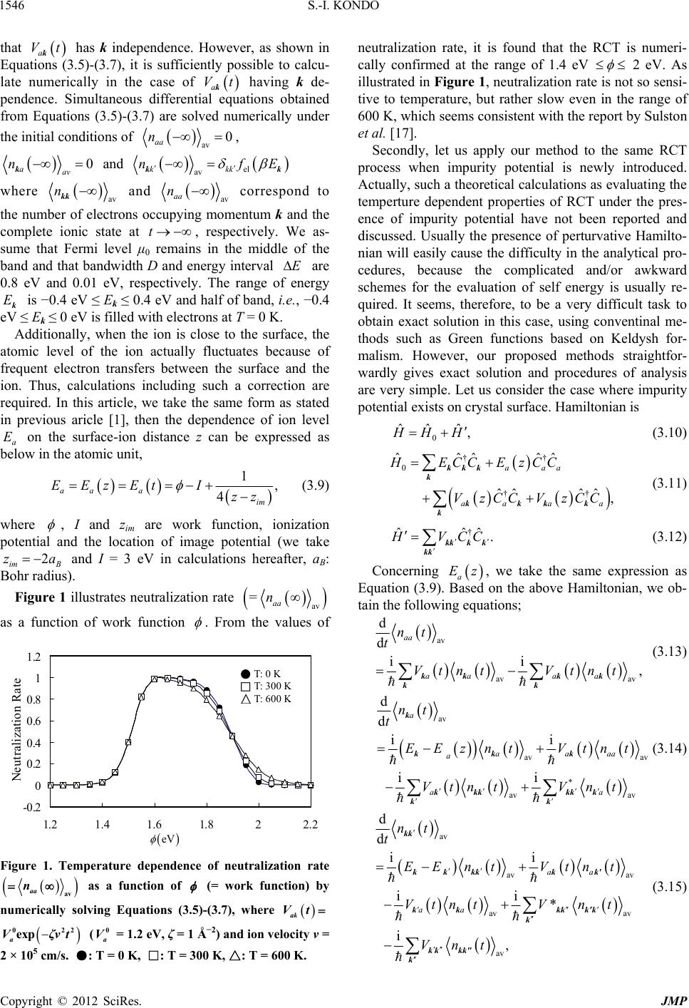 S.-I. KONDO 1546 that a Vt k has k independence. However, as shown in Equations (3.5)-(3.7), it is sufficiently possible to calcu- late numerically in the case of a Vt k having k de- pendence. Simultaneous differential equations obtained from Equations (3.5)-(3.7) are solved numerically under the initial conditions of av aa 0n , 0 aav n k and el av kkk nfE kk where av n kk and av aa n correspond to the number of electrons and t occupying momentum k and the complete ionic state at t, respectively. We as- sume that Fermi level μ0 remains in the middle of the bandat bandwidth D and energy interval E h are 0.8 eV and 0.01 eV, respectively. The range of energy Ek is −0.4 eV ≤ Ek ≤ 0.4 eV and h band, i.e., −0.4 eV ≤ Ek ≤ 0 eV is filled with electrons at T = 0 K. Additionally, when the ion is close to the surface, the alf of actually fluctu because of between theace and the ion. Thus, calculations including such a correction are . In this article, e the sam ous aricle [1he depend atomic level of the ionates frequent electron transfers surf requiredwe take form as stated in previ], then tence of ion level a E on the surface-ion distance z can be expressed as below in the atomic unit, 1, 4 aa a im EEzEtIzz (3.9) ere wh , I and zim are work function, ionization potential and the location of image potential (we take z2 im B a and I = 3 eV in calculations hereafter, aB: Bohr radius). Figure 1 illustrates neutralization rate av =aa n as a function of work function . From the values of -0.2 0 0.2 0.4 eutraliz 0.6 0.8 2 2.2 Nation Ra 1 1.2 te 1.2 1.41.6 1.8 T: 0 K T: 300 K T: 600 igure 1. Temperature dependence of neutralization rate K eV F aa nav as a function of (= work function) by here numerically solving Equations (3.5)-(3.7), w ak Vt ζvt 022 (V= 1.2 eV, ζ = 1 Ålocity v = 2 × 105 cm/s. ●: T = 0 K, □: T = 300 △K, : T = 600 K. neutralization rate, it is found that the RCT is numeri- cally confirmed at the range of 1.4 eV aexpVa 0 −2) and ion ve 2 eV. As illustrated in Figure 1, neutralization rate is not so sensi- tive to temperature, but rather slow even in the range of 600 K, which seems consistent with the report by Sulston et al. [17]. Secondly, let us apply our method to the same RCT process when impurity potential is newly introduced. Actually, such a theoretical calculations as evaluating the temperture dependent properties of RCT under the pre - ence of impurity potential hav not been reported and discussed. Usually the presence of perturvative Hamilto- cedures, bec ly re- obtain exact s r- res s e nian will easily cause the difficulty in the analytical pro- ause the complicated and/or awkward schemes for the evaluation of self energy is usual quired. It seems, therefore, to be a very difficult task to olution in this case, using conventinal me- thods such as Green functions based on Keldysh fo malism. However, our proposed methods straightfor- wardly gives exact solution and proceduof analysis are very simple. Let us consider the case where impurity potential exists on crystal surface. Hamiltonian is 0 ˆˆ ˆ , HH (3.10) †† 0 †† ˆˆ ˆˆ ˆ ˆˆˆˆ, aaa aa aa HECCEz CC Vz CCVz CC kkk k kkkk k (3.11) † ˆˆ ˆ. VCC kkk k kk (3.12) Concerning a Ez, we take the same expression as Equation (3.9). Based on the above Hamiltonian, we ob- tain the following equations; av av av d d ii , aa aa aa nt t VtntVtnt kk kk kk (3.13) av d da nt tk av av aa aa nt Vtnt kk(3.14) * av ii ii a aa EEz Vtnt Vnt k kk k kkk kk av av av d d i i, nt t EE ntVtnt Vnt kk kk k kkk" k av av av av ii * aa aa Vt ntVn t kk k k' kk kkkk k (3.15) i C opyright © 2012 SciRes. JMP 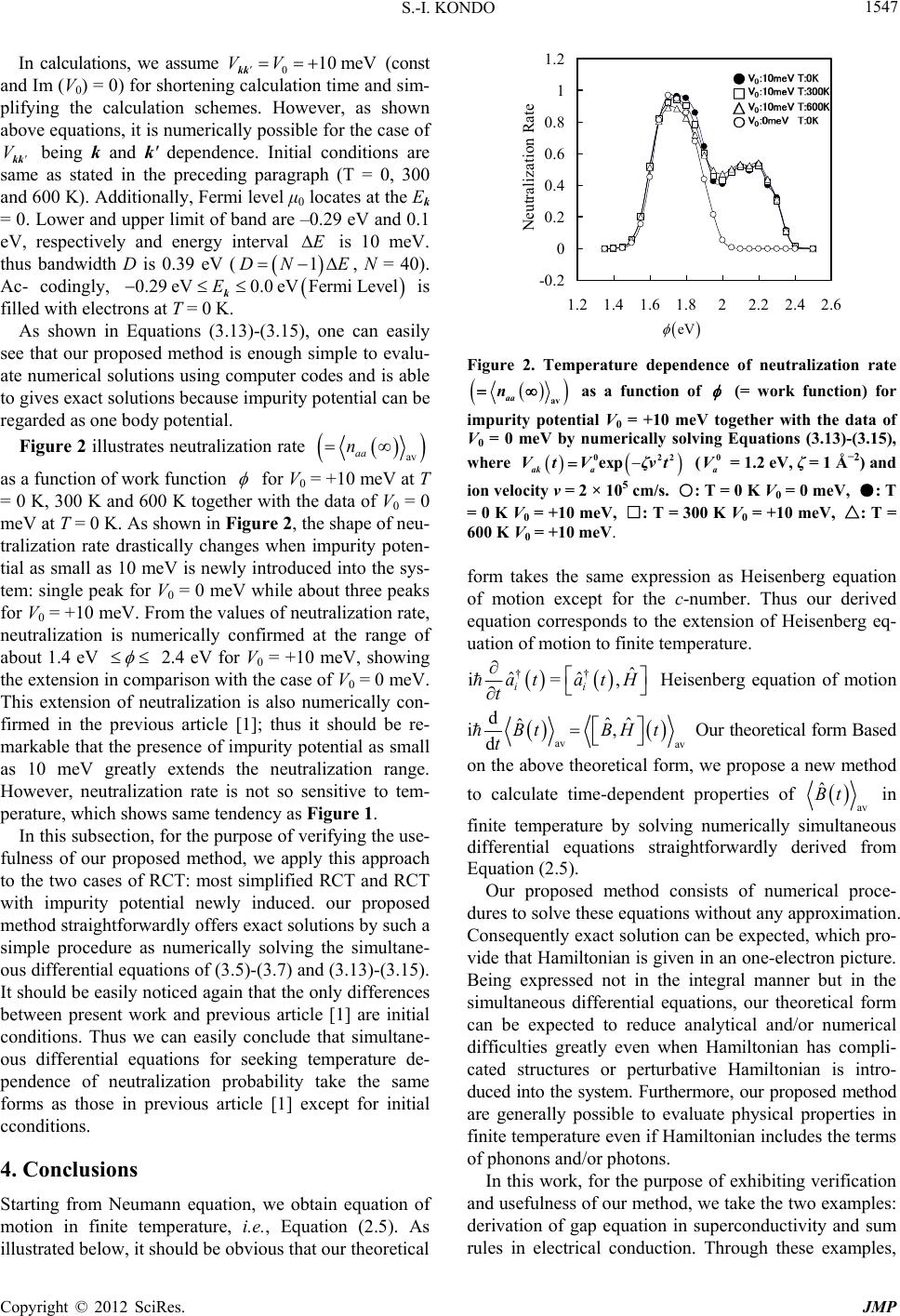 S.-I. KONDO 1547 In calculations,010 meV (const and Im (V0) = 0) lation time and sim plifying the calcus. However, as above equations, it is ble for the case of V kk being kitial conditions are same as stated iragraph (T = 0, 300 and 600 K). Adl μ0 locates at the Ek = 0. Lower an are –0.29 eV a eV, respectivelE is 10 thus bandwidth 1DN E, N = 40). FermiLevel is As shown in Equations (3.13)-(3.15), one can easily see that our proposed method is enough simple to evalu- ate numerical solutions using computer codes and is able to gives exact solutions because impurity potenti regarded as one body potential. Figure 2 illustrates neut we assume VV kk for shortening calcu lation scheme numerically possi and k' dependence. In n the preceding pa ditionally, Fermi leve d upper limit of band y and energy interval D is 0.39 eV ( 0.29 eV0.0E k s at T = 0 K. - shown nd 0.1 meV. Ac- codingly, eV filled with electron al can be ralization rate av aa n as a function ofk function wor for V0 = +10 meV at T = 0 K, 300 K an600 K together with the data of V0 = 0 mgure 2, the shape for d eV at T = 0 K. As shown in Fi of neu- tralization rate drastically changes when impurity poten- tial as small as 10 meV is newly introduced into the sys- tem: single peak for V0 = 0 meV while about three peaks V0 = +10 meV. From the values of neutralization rate, neutralization is numerically confirmed at the range of about 1.4 eV 2.4 eV for V0 = +10 meV, showing the extension in comparison with the case of V0 = 0 meV. This extension of neutralization is also nerically con- firmed in the previous article [uld be re- markable that the all as 10 meV greatly extends t um 1]; thus it sho presence of impurity potential as sm he neutralization range. H mplified RCT and RCT w our proposed owever, neutralization rate is not so sensitive to tem- perature, which shows same tendency as Figure 1. In this subsection, for the purpose of verifying the use- fulness of our proposed method, we apply this approach to the two cases of RCT: most si ith impurity potential newly induced. method straightforwardly offers exact solutions by such a simple procedure as numerically solving the simultane- ous differential equations of (3.5)-(3.7) and (3.13)-(3.15). It should be easily noticed again that the only differences between present work and previous article [1] are initial conditions. Thus we can easily conclude that simultane- ous differential equations for seeking temperature de- pendence of neutralization probability take the same forms as those in previous article [1] except for initial cconditions. 4. Conclusions Starting from Neumann equation, we obtain equation of motion in finite temperature, i.e., Equation (2.5). As illustrated below, it should be obvious that our theoretical -0.2 0 0.2 0.4 0.6 0.8 1 1.2 1.41.6 1.822.2 2.4 2.6 Neutralization Rat 1.2 eV Figure 2. Temperature dependence of neutralization rate aa as a function of n av (= work function) for 0 = +10 meV together with the data of impurity potential V V0 = 0 meV by numerically solving Equations (3.13)-(3.15), where ak a Vt Vζvt 022 exp (a V0 = 1.2 eV, ζ = 1 Å−2) and ion velocity v = 2 × 105 cm/s. ○: T = 0 K V0 = 0 meV, ●: T = 0 K V = +10 meV, □: T = 300 K V = +10 meV, △: T = 0 0 600 K V0 = +10 meV. form takes the same expression as Heisenberg equation of motion except for the c-number. Thus our derived equation corresponds to the extension of Heisenberg eq- uation of motion to finite temperature. ††ˆ ˆˆ i=, ii at atH t Heisenberg equation of motion av av dˆˆˆ i, dBtBH t t Our theoretical form Based on the above theoretical form, we propose a new method to calculate time-dependent perties of rop av finite temperature by solving numerically simultaneous quations straightfowardly derived from Equation (2.5). Our proposed method consists of numerical proce- dures tos without any approximation. Consequently exact solution can be expected, which pro- vide that Hamiltonian is given in an one-electron picture. Being expressed not in the integral manner but in the multaneous differen ˆ Bt in differential er solve these equation tial equations, our theoretical form sical properties in finite temperature even i of phonons and/or photons. In this work, for the purpo and usefulness of our method rules in electrical conduction. Through these examples, si can be expected to reduce analytical and/or numerical difficulties greatly even when Hamiltonian has compli- cated structures or perturbative Hamiltonian is intro- duced into the system. Furthermore, our proposed method are generally possible to evaluate phy f Hamiltonian includes the terms se of exhibiting verification , we take the two examples: derivation of gap equation in superconductivity and sum Copyright © 2012 SciRes. JMP  S.-I. KONDO 1548 our proposed equation seems to be applicablefec- and ef tive in the various fields. It should be noted that our proposed method can be easily applied to the many body problem. For example, when there exists the Coulomb repulsive term between d and d electrons as given as below, †† coulomb ˆˆˆˆ ˆdddd UC C CC , The terms of av ddd nt k and av ddd nt k caused from many body term appear in simultaneous differential equations. In this article, we adopt Hatree Fock approximation avav av ddddd d ntntnt kk , avav av ddddd d ntntnt kk . By introducing such an approximation, we obtain non- linear simultaneous differential equations with showing closed form, which means that numerical solutions are obtainable. However, the above approximation does not include spin cross term such as av dd nt , av dk nt and av dk proximations than Hartree Fock are considered to have the spin cross terms, we could expect such approxima- ts are exrssed as functions of nt . Since more precise ap- ionp eav dd nt , av d nt k, av dd nt and av d nt k or av dd t , n av d n k t , av and dd nt d nt k in the following manner: av av ,, dd d nt nt k avavav ,, ddddd d ntFntnt kk av av ,. dd d nt nt k For further research,it seems more importatnt to find and determine optimized function of F and G. sses, ihtime-de- avav,, dddddd ntGntnt kk n w important s, we ap- ply two cas is the mos quations, w will greatly rede numerical uisad cal- culation timConsequentoposed mseems possible totimate physical properties even if the sys- ime-dependent behaviors. The ded as difficult to analyze be- cause of the presence of impurity potential. The presence of perturbative Hamiltonian such as impurity pottial usually causes comlicated and awkward schemes for the evaluation of self energy. However, our propsoed method straightforwardly deduces the solutions without any as- sumution, which is considered a great merit in analing the case where pertubative Hamiltoniam is introduced. Based on our method, the only differences between gr av Concerning the RCT proceich pendent physical properties playrole es: onet simplified RCT process and the other are the same process but under impurity potential. In analyzing the first case, no integrations as- sociated with time-dependent terms are found in the ob- tained simultaneous differential ehich ucinstabilities, nnces an e. ly our prethod es tem shows complicated t other case is usually regar en yz oud state (T = 0 K) and finite temperature are simple enough to change initial conditions: av aa n 0, av 0 a n k and el av nfE kkkk'k at 0KT whereas 0 aa n , 0 a n k and nE kk'kkk at T = 0 K. Through the analysis of both cases, neutralization process is found to be not so sensitive to temperature up to 600 K while im- purity potential as small as 10 meV greatly changes the neutralization process. In addition, as already stated in the previous article [1], small energy intervals ΔEcan give accurate and reliable calculation results, which means that the number of elec- trons N is large because of ΔNDE (D: band width). Furthermore, assuming that the system consists of N electrons, then numerical solutions of 2 N simultaneous differential equations are required. For example, let us consider actual case. Usually D takes several eV. If we set energy interval Δ1E meV, the value of N is in the range of several thousand, which indicates that we have to solve 106 - 107 simutaneous differential equations. In this article, we adopt algorithm based on the Runge- Kutta-Fehlberg formula and solve numerical 103 simultaneous differential equations, ve a hugdif- equations afrom points of moula ly about 6 × however a fast algorithm to sole number of simultaneous ferentialccurately is strongly desirable the viewre precise simtions. ,” Progress of Theoretical REFERENCES [1] S. Kondo and K. Yamada, “Analysis of Resonance Charge Transfer Neutralization on the Basis of Heisen- berg Equations of Motion Physics, Vol. 122, No. 3, 2009, pp. 713-734. doi:10.1143/PTP.122.713 [2] R. Kubo, “Statistical-Mechanical Theory of Irreversible Processes. I. General Theple Applications to Magnetic and Conduction Problems,” Journal of the Physical Society of Japan, Vol. 12, No. 3, 1957, pp. 570- 586. ory and Sim doi:10.1143/JPSJ.12.570 [3] R. Brako and D. M. Newns, “Charge Exchange in Atom- Surface Scattering: Thrmal versus Quantum Mechanical Non-Adiabaticity,” Surface Science, Vol. 108, No. 2, 1981, pp. 253-270. [4] R. Brako and D. M. Newns, “Theory of Electronic Proc- esses in Atom Scattering from Surfaces,” Reports on Progress in Physics, Vol. 52, No. 6, 1989, pp. 655-698. e C opyright © 2012 SciRes. JMP  S.-I. KONDO Copyright © 2012 SciRes. JMP 1549 doi:10.1088/0034-4885/52/6/001 [5] W. Bloss and D. Hone, “Theory of Charge Exchange Scattering from Surfaces,” Surface Science, Vol. 72, No. 2, 1978, pp. 277-297. [6] H. Winter and R. Zimny, Proceedings of XV ICPEAC Elsevier, Brigh [7] R. Brako, H.wns, “Anisot , ton, 1987. Winter and D. M. Neropic Excitation of Hydrogen 2p after Grazing Ion-Surface Scattering,” Europhysics Letters, Vol. 7, No. 3, 1988, pp. 213-218. doi:10.1209/0295-5075/7/3/005 [8] D. M. Newns, “Self-Consistent Model o Chemisorption,” Physical R f Hydrogen eview, Vol. 178, No. 3, 1969, pp. 1123-1135. doi:10.1103/PhysRev.178.1123 [9] L. V. Keldysh, “Diagram Technique for Nonequilibrium,” Soviet Physics JETP, Vol. 20, No. 4, 1965, pp. 1018- 1026. [10] T. Sakai, M. Sakaue, H. Kasai and A. Okiji, “Theory of Dynamics of Electron Wave Packets in Time-Resolved Two-Photon Photoemission via Image States,” Applied Surface Science, Vol. 169-170, 2001, pp. 57-62. doi:10.1016/S0169-4332(00)00633-4 n 600, No. 10, 2006, pp [11] E. A. García, C. G. Pascual, P. G. Bolcatto, M. C. G. Passeggi and E. C. Goldberg, “Ion Fractions in the Scat- tering of Hydrogen on Different Reconstructed Silico Surfaces,” Surface Science, Vol. . 2195-2206. doi:10.1016/j.susc.2006.03.008 [12] M. Krawiec, M. Jalochowski and M. Kisiel, “High Reso- lution Scanning Tunneling Spectroscopy of Ultrathin Pb Its Va- 1-3, 1996, pp. 145- 603, No. on Si(111)-(6 × 6) Substrate,” Surface Science, Vol. 600, No. 8, 2006, pp. 1641-1645. [13] T. Mii and K. Makoshi, “An Interpolation Formula for Electron Transfer in Atom-Surface Collision and lidity,” Surface Science, Vol. 363, No. 149. [14] E. A. García, M. A. Romero, C. González and E. C. Goldberg, “Neutralization of Li+ Ions Scattered by the Cu(100) and (111) Surfaces: A Localized Picture of the Atom-Surface Interaction,” Surface Science, Vol. 4, 2009, pp. 97-605. doi:10.1016/j.susc.2008.12.022 [15] A. Sindona and G. Falcone, “Evidences of a Double Re- sonant Ionization Mechanism in Sputtering of Metals,” Surface Science, Vol. 529, No. 3, 2003, pp. 471-489. doi:10.1016/S0039-6028(03)00334-0 [16] A. Sindona, P. Riccardi, S. Maletta and G. Falcone, “Double Resonant Neutralization in Hyperthermal Energy Alkali Ion Scattering at Clean Metal Surfaces,” Nuclear Instruments and Method in Physics Research B, Vol. 267, No. 4, 2009, pp. 578-583. doi:10.1016/j.nimb.2008.11.053 [17] K. W. Sulston and F. O. Goodman, “Electronic Bath ap- proach to Thermal Effects in Ion-Surface Scattering,” The Journal of Chemical Physics, Vol. 112, No. 5, 2000, p. 2486.
|