World Journal of Mechanics, 2012, 2, 253-261
doi:10.4236/wjm.2012.25031 Published Online October 2012 (http://www.SciRP.org/journal/wjm)
A Conservative Pressure-Correction Method on Collocated
Grid for Low Mach Number Flows
S. M. Yahya1, S. F. Anwer2, S. Sanghi1
1Department of Applied Mechanics, Indian Institute of Technology, Delhi, India
2Department of Mechanical Engineering, Zakir Husain College of Engineering & Technology,
Aligarh Muslim University, Aligarh, India
Received July 7, 2012; revised August 9, 2012; accepted September 1, 2012
ABSTRACT
A novel extension to SMAC scheme is proposed for variable density flows under low Mach number approximation.
The algorithm is based on a predictor—corrector time integration scheme that employs a projection method for the
momentum equation. A constant-coefficient Poisson equation is solved for the pressure following both the predictor and
corrector steps to satisfy the continuity equation at each time step. The proposed algorithm has second order centrally
differenced convective fluxes with upwinding based on Cell Peclet number while diffusive flux are viscous fourth order
accurate. Spatial discretization is performed on a collocated grid system that offers computational simplicity and
straight forward extension to curvilinear coordinate systems. The algorithm is kinetic energy preserving. Further in this
paper robustness and accuracy are demonstrated by performing test on channel flow with non-Boussinesq condition on
different temperature ratios.
Keywords: LES; Non-Boussinesq; Low Mach Number; Turbulent Flow
1. Introduction
Various flow regimes in industrial devices are of low
speed nature. Such flows are called incompressible, since
the velocities are much smaller than the speed of sound.
In non-reacting incompressible flows without heat trans-
fer, the use of a pressure-correction algorithm has proven
to be accurate and efficient (e.g. [1,2]). Since density
remains constant, no substantial problems are encoun-
tered and the solution is straightforward. The mass con-
servation equation naturally imposes a constraint on the
velocity field. However, if density varies strongly in time
and space, e.g. due to temperature variation, the set of
equations becomes more coupled and an efficient solu-
tion is no longer obvious. Various attempts have been
made to create efficient solution methods. A basic diffi-
culty stems from the acoustic waves in the compressible
formulation. As acoustic waves act at a substantially
smaller time scale than the convective phenomena in low
Mach number flows, the acoustic modes do not signifi-
cantly influence the solution and may be regarded as su-
perfluous. The use of larger time steps, corresponding to
the convective scales, can therefore strongly improve
computational efficiency without loss of relevant infor-
mation.
Furthermore conservation of kinetic energy in numer-
ical methods has become an important issue in large eddy
simulation (LES) and direct numerical simulation (DNS)
of turbulence. Kinetic energy conservation in a finite
difference formulation is not a consequence of discrete
momentum and discrete mass conservation, so conserva-
tion of kinetic energy has to be ensured through careful
design of the finite difference operators. It is known that
dissipative numerical schemes (e.g. up-winding) often
introduce too much artificial damping for use in turbu-
lence simulations, because the energy balance in turbu-
lence is rather delicate. In the case of variable density
flows, not conserving the kinetic energy can also lead to
erroneous temperature and density fields. Much work has
been done in the development of kinetic energy conser-
vation algorithms for incompressible flows (see Vasilyev
[3]; Gullbrand [4]; Morinishi et al. [5]), but there has
been less work on variable density or compressible flows
(see Nicoud [6] and Lessani [7]). In low-speed turbulent
channel flow applications, the low Mach-number, vari-
able-density approximation of the Navier-Stokes equa-
tions is a good basis for simulation, as it supports large
density variations while eliminating acoustic waves. This
eliminates the need for extremely small time steps driven
by the acoustics. This means that the arising velocities
are much smaller than the speed of sound, so that density
variations due to pressure variations can be neglected. In
those so-called low Mach number flows, an efficient way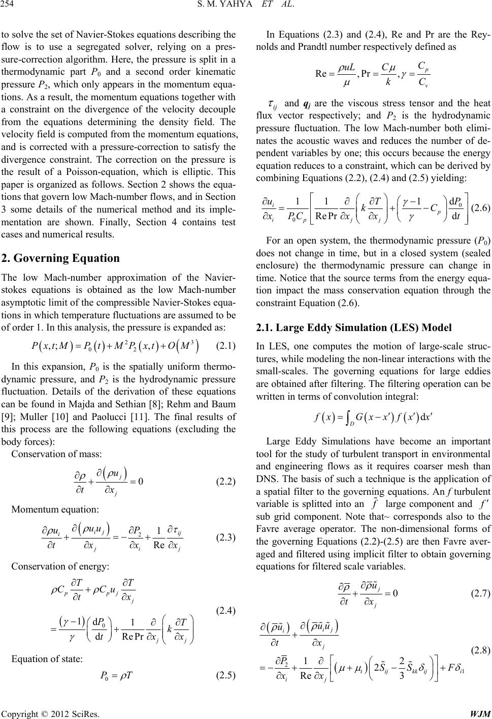

S. M. YAHYA ET AL.
254
to solve the set of Navier-Stokes equations describing the
flow is to use a segregated solver, relying on a pres-
sure-correction algorithm. Here, the pressure is split in a
thermodynamic part P0 and a second order kinematic
pressure P2, which only appears in the momentum equa-
tions. As a result, the momentum equations together with
a constraint on the divergence of the velocity decouple
from the equations determining the density field. The
velocity field is computed from the momentum equations,
and is corrected with a pressure-correction to satisfy the
divergence constraint. The correction on the pressure is
the result of a Poisson-equation, which is elliptic. This
paper is organized as follows. Section 2 shows the equa-
tions that govern low Mach-number flows, and in Section
3 some details of the numerical method and its imple-
mentation are shown. Finally, Section 4 contains test
cases and numerical results.
2. Governing Equation
The low Mach-number approximation of the Navier-
stokes equations is obtained as the low Mach-number
asymptotic limit of the compressible Navier-Stokes equa-
tions in which temperature fluctuations are assumed to be
of order 1. In this analysis, the pressure is expanded as:
 

23
02
,; ,PxtMP tMPxtOM 

(2.1)
In this expansion, P0 is the spatially uniform thermo-
dynamic pressure, and P2 is the hydrodynamic pressure
fluctuation. Details of the derivation of these equations
can be found in Majda and Sethian [8]; Rehm and Baum
[9]; Muller [10] and Paolucci [11]. The final results of
this process are the following equations (excluding the
body forces):
Conservation of mass:

0
j
j
u
tx





 (2.2)
Momentum equation:

21
Re
ij ij
i
j
ij
uu
uP
tx x

x





 
(2.3)
Conservation of energy:

0
1d1
dRePr
ppj
j
j
j
TT
CCu
tx
PT
k
tx











 

 
x
(2.4)
Equation of state:
0
PT

 (2.5)
In Equations (2.3) and (2.4), Re and Pr are the Rey-
nolds and Prandtl number respectively defined as
Re, Pr,
p
v
C
uL C
kC




ij

and qj are the viscous stress tensor and the heat
flux vector respectively; and P2 is the hydrodynamic
pressure fluctuation. The low Mach-number both elimi-
nates the acoustic waves and reduces the number of de-
pendent variables by one; this occurs because the energy
equation reduces to a constraint, which can be derived by
combining Equations (2.2), (2.4) and (2.5) yielding:
0
0
d 11 1
Re Prd
i
p
ip jj
uP T
kC
x
PCx xt





  












(2.6)
For an open system, the thermodynamic pressure (P0)
does not change in time, but in a closed system (sealed
enclosure) the thermodynamic pressure can change in
time. Notice that the source terms from the energy equa-
tion impact the mass conservation equation through the
constraint Equation (2.6).
2.1. Large Eddy Simulation (LES) Model
In LES, one computes the motion of large-scale struc-
tures, while modeling the non-linear interactions with the
small-scales. The governing equations for large eddies
are obtained after filtering. The filtering operation can be
written in terms of convolution integral:




d
D
f
xGxxfx


x

Large Eddy Simulations have become an important
tool for the study of turbulent transport in environmental
and engineering flows as it requires coarser mesh than
DNS. The basis of such a technique is the application of
a spatial filter to the governing equations. An f turbulent
variable is splitted into an
f
 large component and
f

sub grid component. Note that~ corresponds also to the
Favre average operator. The non-dimensional forms of
the governing Equations (2.2)-(2.5) are then Favre aver-
aged and filtered using implicit filter to obtain governing
equations for filtered scale variables.
0
j
j
u
tx







%
(2.7)




2
1
12
2
Re 3
ij
i
j
tij kkij
ij
uu
u
tx
PSS F
xx


i





 

 
 
 

%%
%
%%
(2.8)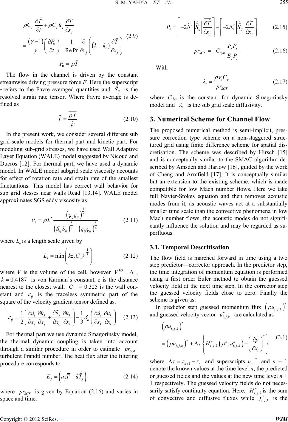

S. M. YAHYA ET AL. 255


0
11
Re Pr
ppj
j
t
j
j
TT
CCu
tx
PT
kk
tx









 

 

 
%%
%
%
x
(2.9)
0
PT

%
The flow in the channel is driven by the constant
streamwise driving pressure force F. Here the superscript
~refers to the Favre averaged quantities and ij is the
resolved strain rate tensor. Where Favre average is de-
fined as
S
%
f
f



%
% (2.10)
In the present work, we consider several different sub
grid-scale models for thermal part and kinetic part. For
modeling sub-grid stresses, we have used Wall Adaptive
Layer Equation (WALE) model suggested by Nicoud and
Ducros [12]. For thermal part, we have used a dynamic
model. In WALE model subgrid scale viscosity accounts
for effect of rotation rate and strain rate of the smallest
fluctuations. This model has correct wall behavior for
sub grid stesses near walls Read [13,14]. WALE model
approximates SGS eddy viscosity as


3
2
2
5
24
ij ij
ts
ijijij ij
L
SS





5
(2.11)
where Ls is a length scale given by
1
3
min ,
s
LkzCV




w


(2.12)
where V is the volume of the cell, however 13
t
V

,
is von Karman’s constant, z is the distance
nearest to the closest wall, w = 0.325 is the wall con-
stant and ij
0.4187k
C

is the traceless symmetric part of the
square of the velocity gradient tensor defined as.
11
23
j
ik klk
ij ij
kj kikl
u
uu uuu
x
xxx xx

 
 




 


%
%% %%%


(2.13)
For thermal part we use dynamic Smagorinsky model,
the thermal dynamic coupling is taken into account
through a similar procedure in order to estimate SGC
turbulent Prandtl number. The heat flux after the filtering
procedure corresponds to
pr

ˆ
ˆ
j
j
EuTuT
%
%j
(2.14)
where SGS is given by Equation (2.16) and varies in
space and time.
pr
22
ˆ
ˆˆ
ˆ
22
jij tij
j
j
T
PS S
T
x
x




 






%
%%


(2.15)
d
j
j
SGS yn
j
j
PP
prC EP  (2.16)
With
tp
t
SGS
C
pr


 (2.17)
where Cdyn is the constant for dynamic Smagorinsky
model and t

is the sub grid scale diffusivity.
3. Numerical Scheme for Channel Flow
The proposed numerical method is semi-implicit, pres-
sure correction type scheme on a non-staggered struc-
tured grid using finite difference scheme for spatial dis-
cretisation. The scheme was described by Hirsch [15]
and is conceptually similar to the SMAC algorithm de-
scribed by Amsden and Harlow [16], guided by the work
of Cheng and Armfield [17]. It is conceptually similar
but an extension to the existing scheme, which is made
compatible for low Mach number flows. Here we take
full Navier-Stokes equation and then removes acoustic
modes from it, as acoustic waves act at a substantially
smaller time scale than the convective phenomena in low
Mach number flows, the acoustic modes do not signifi-
cantly influence the solution and may be regarded as su-
perfluous.
3.1. Temporal Descritisation
The flow field is marched forward in time using a two
step predictor—corrector approach. In the predictor step,
the time integration of momentum equation is performed
using a first order Euler method to obtain the guessed
velocity field at the next time step. In the corrector step
the guessed velocity fields close to zero. Finally the
scheme is given as:
In predictor step guessed momentum flux


,,ijk
u 

and guessed velocity vector are calculated as
,,ijk
u


 
,,
,,,,,,
,
ijk
n
nnnn
ijkijk ijk
i
u
p
uHu
x









 

 





(3.1)
where 1nn





and superscripts n, *, and n + 1
denote the known values at the time level n, the predicted
or guessed fields and the values at the new time level n +
1 respectively. The guessed velocity fields do not neces-
sarily satisfy continuity equation. Here, ,, is the sum
of convective and diffusive fluxes while
n
ij k
H
n
,,ij k
f
is the

S. M. YAHYA ET AL.
256
sum of convective and heat transfer fluxes at time level
“n”. The predicted value for the temperature T* is calcu-
lated from Equation (2.4) based on previous values at
time level n,

1
00
,, ,,,,,,
,, 1
nn
nnnnn
ijk ijkijkijk
n
p
pp
TTf uT
C






 
 







(3.2
Guessed thermodynamic pressure and guessed de
fie
)
nsity
ld would be
0
0d
M
PV
T




0
P
T





In this step guessed velocity field obtained in the pre-
dictor step is corrected in a continuity preserving manner,
firstly we define correction flux and correction pressure


11 nn
,, ,,
,, ,, ij
k ijk
ijk ijk
F
uuu FF     
 

 (3.3)
And
(3.4)
The velocity and temperature field at tim
th
1
,,,,
nn
ijk ijk
PP P


e level n + 1
at satisfies continuity is coupled to the pressure field at
anew time level n + 1 through a semi explicit discretisa-
tion in time of the momentum equations. This is given
by,

1
1*
00
,, ,,,,,,
,, 1
nn
nn nnn
i jkijki jki jk
n
p
pp
TTf uT
C






 
 
 







 



(3.5)


1n
1
,, ,,,, ,,
,
nn
nn
n
ijkijkijk ijk
i
p
uu Hu
x

 


 
 




(3.6)
The relationship between velocity and pressure co
tion (P') can be obtained by subtracting Equation
fr


rrec-
(3.1)
om (3.6). This yields
1
,,
n
ijk
P
F,,
ijk
i
F
x
 


 


i
P
F
x



  (3.7)
Taking divergence of the above
the discrete divergence operator defined as below
Equation (3.7) with
d
i
x




1
,, ,,
.
n
dijkijkd
i
P
FF
21
d
PF





Now using continuity equation and defined correction
flux we get
1
21n
P








 


 

 



where below mentioned value of density is used
son equation

(3.8)
in Pois-
10
0d
nM
PV

.
x

 






1 n
T



1
10
1
n
n
n
P
T





For a closed system, like ours, the thodynamic
pressure po is calculated by using
erm
0
0d
n
n
M
PV
T


10
0d
nM
PV

1 n
T

1
000
d
d
nn
PPP
t 


 (3.9)
3.2. Spatial Descritisation
The spatial discretization is performed using finite dif-
cated mesh with a Carte-
-winding scheme employs
ference methodology on a collo
sian coordinate system. The up
two points in upstream and one point on the downstream
side of the grid under-consideration. Convective fluxes
are second order centrally differenced; the choice be-
tween up-winding and central differencing is made on
the basis of cell Peclet number while diffusive fluxes are
viscous fourth order accurate. The discrete Poisson equa-
tion is differenced as
11
,, ,, 1
1
i
PPP
xx x


22
ijk ijk
x x



 


 



 

 




where

(3.10)
1, ,, ,
1,, 2
2
ijk ijk
ijk
PP
P
xx 






 


 (3.11)
,, 1,,jk
1,,3
2
ij k i
ijk
PP
P
xx



 


 



11 1
123
,,
22
iiii ii1
2
x
xxxx
xxx 
x



 

Convective flux are second order centrally differenced
given below

 
111
,,
2
nn
nn
2
nn
xx 
n
ii
niii RL
ijk
uuuu TTT
fk



 (3.12)

S. M. YAHYA ET AL. 257
where the subscripts R and L indicate extrapolated values
at the right and left face of the control volume. F
order upwinding, and positive values of the velocity, this
or first
means

11
22
Rii
uu 

 and

11
22
Lii
uu 


with averaged face density values:

11
2
ii
i



y averaging:
2
The node velocities are calculated b
11
22
iii


2uu u



Diffusive fluxes are viscous fourth order accurate
which is calculated as follows:
1, ,,,
,,
1
Re
ijk ijk
ijk
Hx


 

2, ,1,,1,,2, ,4
,,
88
12
ijkijkijk ijk
ijk
uuuu
Ox
x


  


(3.13)
 
4. Results and Discussion
Three numerical experiments were performed in o
ts implementation. We
for TLES (thermal large
rder to
test the numerical scheme and i
used self made FORTRAN code
eddy simulation). A mesh of size 96 × 96 × 96 is used for
simulation purpose, uniform meshes are used in the
stream-wise and span-wise directions and a non-uniform
mesh with hyperbolic tangent distribution is used in the
wall-normal direction. For the velocities, no slip bound-
ary condition was used on the top and bottom walls and
periodic boundary condition was used in x-y direction.
The temperatures on the hot and cold walls were set ac-
cording to R

. Viscosity was calculated using Suther-
lands law with reference at Tc. The reference Reynolds
number based on the reference velocity and channel half
width is keponstant at 2800 while the Prandtl number
is fixed at 0.71.
First, a 1D convection-diffusion problem was set to
test spatial and temporal convergence in a variable den-
sity case. Second
t c
, a 2D inviscid solenoidal velocity field
w
lem for this experiment is a temperature
m-
-
main was the interval [0, 1]. The initial temperature pro-
as used to test kinetic energy conservation. Finally, a
3D turbulent channel flow with large temperature gradi-
ent is used.
4.1. Spatial and Temporal Convergence in 1D
The test prob
profile that will be convected in the x-direction. For si
plicity the flow was assumed to be inviscid and the do
file is a Gaussian given by equation.

2
0.5
295 50exp0.05
x
Tk 


 





(4.1)
The velocity in the x-direction (u) was set equal to 1;
the hydrodynamic pressure was set to 0 Pa and t
modynamic pressure was set to 1. The work
assumed to be air so that its thermal conductivity (k)
co
l steady
quation (4.2).
he ther-
ing fluid was
uld be estimated from polynomial correlations. Since
the thermal diffusivity of air is O (1 × 10E−05), the
global Peclet number is very high O (1 × 10E−05). For
the spatial convergence the grid was changed from 100,
200, 400 to 800 nodes while the time step was held in
0.00125 so that the CFL number changed from 0.125 to 1.
For the temporal convergence the mesh was held in 100
grid points and the time was changed from 0.005 to
0.000625 so that the CFL number changed from 0.5 to
0.0625. Figure 1 shows the profile of velocity at t = 1 for
four different time steps. The velocity induced by the
diffusion process was of the order 1 × 10−6. The shape of
the u-velocity profile is in agreement with the theory and
what is expected from Equation (4.1). Table 1 summa-
rizes the numerical results from this experiment.
4.2. Kinetic Energy Conservation
For this numerical experiment a 2-dimensional rectangu-
lar domain [0, 1] × [0, 1] is used, with an initia
state solenoidal velocity field given by E



 
 
,cos2πsin2π
,sin2πcos 2π
uxyx y
vxyx y

 (4.2)
The temperature field was set as a Gaussian random field
with a mean value of 397 K and a root mean square fluc-
tuation of 57 K. The density field can be
the equation of state. Using Equation (4.2) and the initial
computed from
random density field, the initial kinetic energy can be
computed (KE0 = 0.2274 J). A mesh of 24 × 24 points
was used, so that Δx = Δy = 4.2e−02. According to Ni-
coud [6], the integration time for this numerical experi-
ment is given by Equation (4.3).
Figure 1. “u” velocity profile.

S. M. YAHYA ET AL.
258
0
0.125 0.3125 L
ts
KE
 (4.3)
Table 2 and Figure 2 show the results for this ex-
periment. It is evident that the scheme conserves global
kinetic energy, so that the divergence-free constraint is
recovered in the inviscid limit.
The error in Table 2 was calculated using the ratio
between the difference in the initial and final kinetic en-
ergy i.e.
0
0
ERROR
f
K
EKE
4.3. 3D Channel Flow Simulation
In
subsection, we consider turbulent flow in a
channel whose walls are kept at differet temperatures.
This problem is treated numerically withhe help of LES.
Let x, y and z, denote the stream-wise, span-wise and
imensions of the
δ being the half
Δy × Δz = 33 × 11 × [05:11].
U
KE

this section, we present detailed numerical results
from the test problems that we considered in order to
check the robustness and accuracy of the proposed algo-
rithm. This is the case of large-eddy simulation (LES) of
non-isothermal, turbulent channel flow with strong tem-
perature gradients due to the temperature difference be-
tween the two walls.
In this
n
t
normal directions, respectively. The d
domain are 4 πδ × 4/3 πδ × 2δ, with
width of the channel. The walls of the channel are normal
to the z direction and are held at constant temperature.
The boundaries of the domain normal to the x and y di-
rections are periodic in nature. Therefore, the total mass
of the system is conserved, i.e., this is an example of
flow in a closed domain. A mesh of 643 points is used in
such a way that Δx+ × + +
niform meshes are used in the stream-wise and span-
ise directions and a non-uniform mesh with hyperbolic
Table 1. Spatial and temporal convergence rates.
u v T
Spatial 1.971 1.954 1.881
Temporal 0.967 0.942 0.977
Table 2. Numerical results from KE conservation.
Δt CFL KE0 KEf ERROR
0.04166 1 0.2274 0.226879 2.59 × 10e−03
0.02083 0.5 0.2274 0.226891 2.54 × 10e−03
0.0 03
0.002083 0.05 0.2274 0.226921 2.40 × 10e−03
0.00046 0.01 0.226 2.38 × 103
04166 0.1 0.2274 0.226918 2.42 × 10e−
160.2274 9270e−
Figure 2. Error of the KE as a function of CFL.
tangent distribution is used in the wall-normal direction.
The Wall-Adapting Local Eddy-viscosity (W-ALE) model
(Nicoud [12]) is used for modeling the eddy viscosity
and dynamic Smagorinsky method is used to model tur-
bulent heat flux. In the homogeneous directions, the
convective terms of the momentum and energy equations
are calculated using hybrid type upwind. The multi- grid
algorithm (Jameson [18]) is used to solve the con-
stant-coefficient pressure Poisson equation. Let Th and Tc
denote the temperatures of the hot and cold walls, re-
spectively. Two different cases, corresponding to diffe
ent wSpe-
ifically,
r-
all temperature ratios, are considered herein.
cR

= 1.01 and R

= 2. Here, R

= hc TT.
For all the simulations

2
mhc
TTT is used to ini-
tialize the flow field. Table 1 represents important simu-
lation parameters. For comparison purposes between our
results and with the Direct Numerical Simulations (DNS)
data, we used a molecular Prandtl number of 0.7 for the
first case (hc
TT = 1.01) and Sutherland law for the case
(hc TT= 2). The R

= 1.01 results are compared with the
DNS of Kim et al. [19] and Lessani [20], while R

= 2
results are compared with DNS of Nicoud [21] as shown
in Table 3.
Figure 3 shows that Rθ = 1.01 is in good agreement
with previous incompressible DNS (Kim et al., [19]) for
the mean ocity profile. Te expected (fothe fn
Reynolds number conside-wall u+ = 2.5
ln(y+) + 5.5 is recovered. The viscous sub layer is also
well resolved as shown in Figure 3. Figure 4 shows a
good agreement with previous incompressible DNS (Kim
et al., [19]) for the three velocity fluctuations and the
Reynolds sheastess. For any instantaneous variable
velhr rictio
ered) law-of-th
r

,

denotes the time and space averaged field. Space
averaging is performed in the homogenous direction a
fluctuating field is defined as
nd


 , hence
12
rms



. The mean stream-wise velocity is
u
uu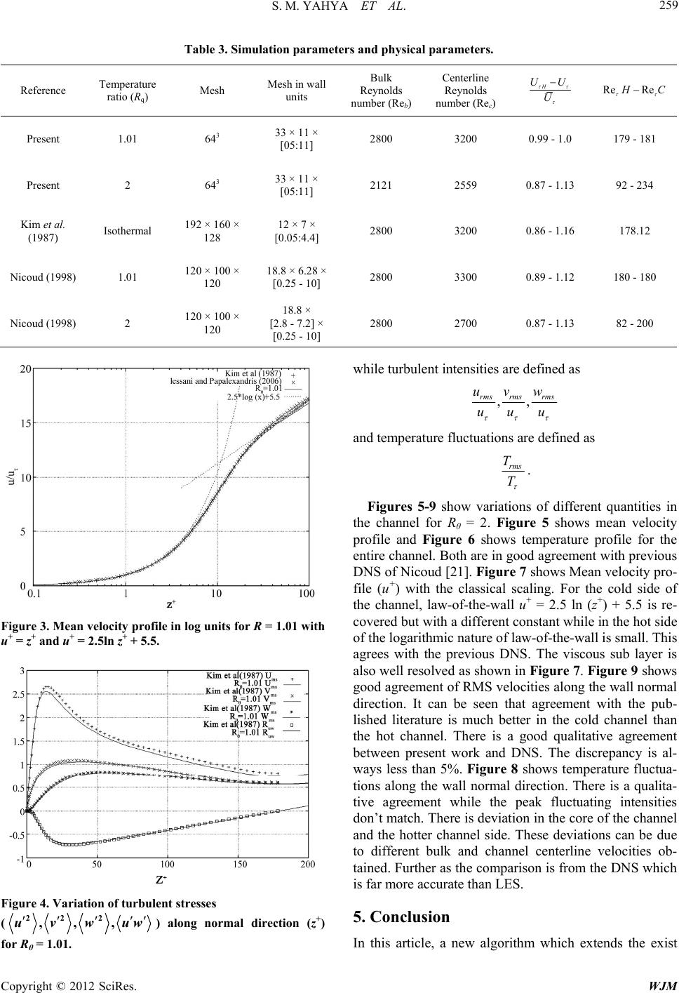



S. M. YAHYA ET AL.
259
ter
Bulk
Reynolds
number (Reb) number (Rec)
Table 3. Simulation parames and physical parameters.
Reference Temperature
ratio (Rq) Mesh Mesh in wall units
Centerline
Reynolds H
UU
U


 Re
H
Re C



Present 1.01 643 33 × 11
[05:11]
×2800 3200 0.99 - 1.0 179 - 181
Present 2 643 33 × 11 × 0.87 - 1.13 92 - 234
Kim et al.
(1987) Isothermal 192 × 160 × 128
12 × 7 ×
[0.05:4.4] 2800 3200 0.86 - 1.16 178.12
Nicoud (1998) 1.01 120 × 100 ×
120
18.
[0.25 - 10] 2800 3300 0.89 - 1.12 180 - 180
Nicoud (1998) 2 120 × 100 ×
120 [2.8 - 7.2] ×
[
2800 2700 0.87 - 1.13 82 - 200
[05:11] 2121 2559
8 × 6.28 ×
18.8 ×
0.25 - 10]
Figure 3. Mean velocity profile in log units for R = 1.01 with
u+ = z+ and u+ = 2.5ln z+ + 5.5.
Figure 4. Variation of turbulent stresses
( uvw uw
22 2
,, ,
for Rθ = 1.01.

) along normal direction (z+)
while turbulent intensities are defined as
,,
rms
w
rms
urms v
uuu


an perature f as d temluctuations are defined
rms
T
T

.
Figures 5-9 show variations of different quantities in
the channel for Rθ = 2. Figure 5 shows mean velocity
profile and Figure 6 shows temperature profile for the
entire channel. Both are in good agreement with previous
DNS of Nicoud [21]. Figure 7 shows Mean velocity pro-
file (u+) with the classical scaling. For the cold side of
the channel, law-of-the-wall u+ = 2.5 ln (z+) + 5.5 is re-
covered but with a different constant while in the hot side
of the logarithmic nature of law-of-the-wall is small. This
agrees with the previous DNS. The viscous sub layer is
also well resolved as shown in Figure 7. Figure 9 shows
good agreement of RMS velocities along the wall norm
direction. It can be seen that agreement with the pub-
old channel than
e hot channel. There is
resent work and DNS. The discrepancy is al-
erature fluctua-
tions along the wall normal direction. There is a qualita-
tive agreement while the peak fltuating intensities
don’t match. There is deviation in the core of the channel
s can be due
elocities ob-
tained. Further as the comparis is from the DNS which
is far more accurate than LES.
al
lished literature is much better in the c
th a good qualitative agreement
between p
ways less than 5%. Figure 8 shows temp
uc
and the hotter channel side. These deviation
to different bulk and channel centerline v
on
5. Conclusion
In this article, a new algorithm which extends the exist

S. M. YAHYA ET AL.
260
Figure 5. Mean Stream-wise velocity profile normalized
with maximum velocity for the entire channel.
Figure 6. Mean Temperature for c
TT
TΔ for the entire
channel along wall normal direction, for Rθ = 2.
Figure 7. Mean velocity profile in log units along the chan-
nel for Rθ = 2.
ing SMAC scheme for low Mach number, variable den-
sity flows has been presented. This algorithm can be ap-
plied to both open and closed domains. It is based on
two-stage predictor—corrector method. This algorithm is
a
Figure 8. Variation of Trms along the wall normal direction
(z+) for Rθ = 2.
Figure 9. Variation of RMS velocities along the wall normal
direction (z) for Rθ = 2.
particularly useful for unsteady flows with strong tem-
perature gradients. A constant-coefficient Poisson equa-
tion, which is computationally more efficient than the
variable-coefficient one, is solved for the pressure. A
collocated grid is used for spatial discretization and not a
ty and straightforward extension to curvi-
near coordinate systems. The odd-even decoupling prob-
lem is avoided by using smartly a continuity equation in
conjunction with correction flux. The robustness and
accuracy of the algorithm have been assessed through
simulations of three test problems; 1D convection-diffu-
sion problem, 2D steady state solenoidal velocity distri-
bution for conservation of kinetic energy and finally the
turbulent channel flow with temperature gradients. The
results obtained with the proposed algorithm are in very
good agreement with the ones reported in earlier studies.
The algorithm has a moderate computational cost for
solving the Poisson-equation and is stable for high den-
sity ratios (at least up to a factor of 10). Though in the
examples shown in this paper, P0 was always a constan
staggered one because collocated grids offer computa-
tional simplici
li
t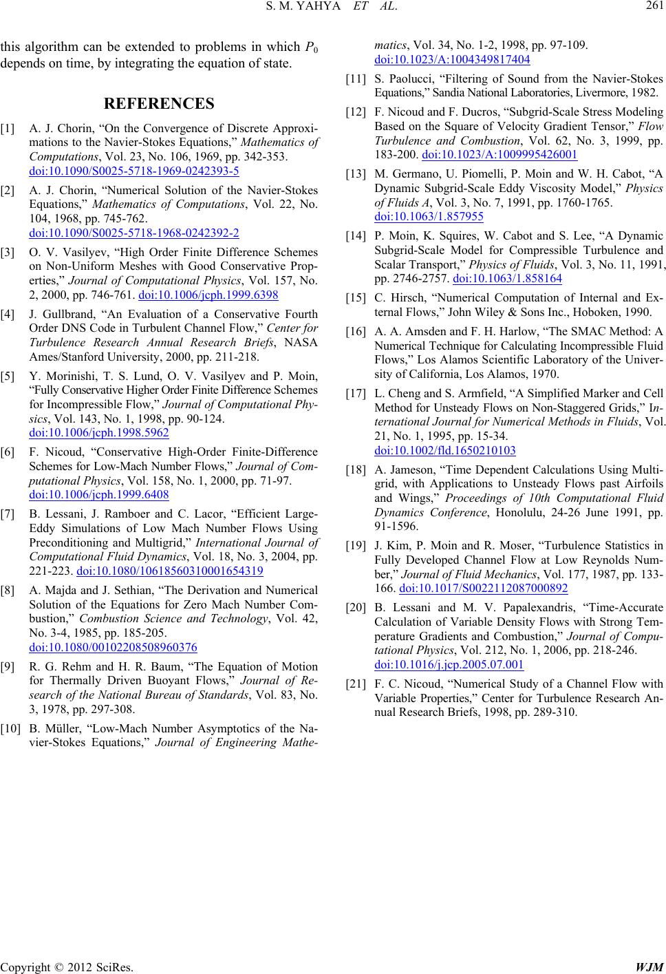

S. M. YAHYA ET AL.
261
egrating the equation of state.
this algorithm can be extended to problems in which P0
depends on time, by int
REFERENCES
[1] A. J. Chorin, “On the Convergence of Discrete Approxi-
mations to the Navier-Stokes Equations,” Mathematics of
Computations, Vol. 23, No. 106, 1969, pp. 342-353.
doi:10.1090/S0025-5718-1969-0242393-5
[2] A. J. Chorin, “Numerical Solution of the Navier-Stokes
Equations,” Mathematics of Computations, Vol. 22, No.
104, 1968, pp. 745-762.
doi:10.1090/S0025-5718-1968-0242392-2
[3] O. V. Vasilyev, “High Order Finite Difference Schemes
on Non-Uniform Meshes with Good Conservative Prop-
erties,” Journal of Computational Physics, Vol. 157, No.
2, 2000, pp. 746-761. doi:10.1006/jcph.1999.6398
[4] J. Gullbrand, “An Evaluation of a Conservative Fourth
Order DNS Code in Turbulent Channel Flow,” Center for
Turbulence Research Annual Research Briefs, NASA
Ames/Stanford University, 2000, pp. 211-218.
[5] Y. Morinishi, T. S. Lund, O. V. Vasilyev and P. Moin,
“Fully Conservative Higher Order Finite Difference Schemes
for Incompressible Flow,” Journal of Computational Phy-
sics, Vol. 143, No. 1, 1998, pp. 90-124.
doi:10.1006/jcph.1998.5962
[6] F. Nicoud, “Conservative High-Order Finite-Difference
Schemes for Low-Mach Number Flows,” Journal of Com-
putational Physics, Vol. 158, No. 1, 2000, pp. 71-97.
doi:10.1006/jc ph.1999.6408
[7] B. Lessani, J. Ramboer and C. Lacor, “Efficient Large-
Eddy Simulations of Low Mach Number Flows Using
Preconditioning and Multigrid,” International Journal of
Computational Fluid Dynamics, Vol. 18, No. 3, 2004,
221-223.
pp.
doi:10.1080/10618560310001654319
logy, Vol.
[8] A. Majda and J. Sethian, “The Derivation and Numerical
Solution of the Equations for Zero Mach Number Com-
bustion,” Combustion Science and Techno
No. 3-4, 1985, pp. 185-205.
42,
doi:10.1080/00102208508960376
[9] R. G. Rehm and H. R. Baum, “The Equation of Motion
for Thermally Driven Buoyant Flows,” Journal of Re-
search of the National Bureau of Standards, Vol. 83, No.
3, 1978, pp. 297-308.
[10] B. Müller, “Low-Mach Number Asymptotics of the Na-
vier-Stokes Equations,” Journal of Engineering Mathe-
matics, Vol. 34, No. 1-2, 1998, pp. 97-109.
doi:10.1023/A:1004349817404
[11] S. Paolucci, “Filtering of Sound from the Navier-Stokes
. 3, 1999, pp.
6001
Equations,” Sandia National Laboratories, Livermore, 1982.
[12] F. Nicoud and F. Ducros, “Subgrid-Scale Stress Modeling
Based on the Square of Velocity Gradient Tensor,” Flow
Turbulence and Combustion, Vol. 62, No
183-200. doi:10.1023/A:100999542
[13] M. Germano, U. Piomelli, P. Moin and W. H. Cabot, “A
Dynamic Subgrid-Scale Eddy Viscosity Model,” Physics
of Fluids A, Vol. 3, No. 7, 1991, pp. 1760-1765.
doi:10.1063/1.857955
[14] P. Moin, K. Squires, W. Cabot and S. Lee, “A Dynamic
Subgrid-Scale Model for Compressible Turbulence and
Scalar Transport,” Physics of Fluids, Vol. 3,
pp. 2746-2757.
No. 11, 1991,
8164doi:10.1063/1.85
ids, Vol.
34.
[15] C. Hirsch, “Numerical Computation of Internal and Ex-
ternal Flows,” John Wiley & Sons Inc., Hoboken, 1990.
[16] A. A. Amsden and F. H. Harlow, “The SMAC Method: A
Numerical Technique for Calculating Incompressible Fluid
Flows,” Los Alamos Scientific Laboratory of the Univer-
sity of California, Los Alamos, 1970.
[17] L. Cheng and S. Armfield, “A Simplified Marker and Cell
Method for Unsteady Flows on Non-Staggered Grids,” In-
ternational Journal for Numerical Methods in Flu
21, No. 1, 1995, pp. 15-
doi:10.1002/fld.1650210103
[18] A. Jameson, “Time Dependent Calculations Using Multi-
grid, with Applications to Unsteady Flows past Airfoils
and Wings,” Proceedings of 10th Computational Fluid
Dynamics Conference, Honolulu, 24-26 June 1991, pp.
91-1596.
[19] J. Kim, P. Moin and R. Moser, “Turbulence Statistics in
Fully Developed Channel Flow at Low Reynolds Num-
ber,” Journal of Fluid Mechanics, Vol. 177, 1987, pp. 133-
166. doi:10.1017/S0022112087000892
o. 1, 2006, pp. 218-246.
[20] B. Lessani and M. V. Papalexandris, “Time-Accurate
Calculation of Variable Density Flows with Strong Tem-
perature Gradients and Combustion,” Journal of Compu-
tational Physics, Vol. 212, N
doi:10.1016/j.jcp.2005.07.001
[21] F. C. Nicoud, “Numerical Study of a Channel Flow with
Variable Properties,” Center for Turbulence Research An-
nual Research Briefs, 1998, pp. 289-310.