 World Journal of Mechanics, 2012, 2, 246-252 doi:10.4236/wjm.2012.25030 Published Online October 2012 (http://www.SciRP.org/journal/wjm) Any Hamiltonian System Is Locally Equivalent to a Free Particle Elizabeth Galindo-Linares1, Esperanza Navarro-Morales1, Gilberto Silva-Ortigoza1*, Román Suárez-Xique1, Magdalena Marciano-Melchor2, Ramón Silva-Ortigoza2, Edwin Román-Hernández3 1Facultad de Ciencias Físico Matemáticas, Benemérita Universidad Autónoma de Puebla, Puebla, México 2CIDETEC-IPN, Departamento de Posgrado, Área de Mecatrónica, Unidad Profesional Adolfo López Mateos, México City, México 3Departamento de Matemáticas Aplicadas, Universidad del Istmo, Guatemala, México Email: *gsilva@fcfm.buap.mx Received July 19, 2012; revised August 16, 2012; accepted August 26, 2012 ABSTRACT In this work we use the Hamilton-Jacobi theo ry to show that locally all the Hamiltonian systems with n degrees of free- dom are equivalent. That is, there is a canonical transformation connecting two arbitrary Hamiltonian systems with the same number of degrees of freedom. This result in particular implies that locally all the Hamiltonian systems are equivalent to that of a free particle. We illustrate our result with two particular examples; first we show that the one-dimensional free particle is locally equivalent to the one-dimensional harmonic oscillator and second that the two-dimensional free particle is locally equivalent to the two-dimensional Kepler problem. Keywords: Hamiltonian System; Canonical Transformation 1. Introduction In the Lagrangian formulation of classical mechanics to each mechanical system with n degrees of freedom there is associated an abstract space of dimension n, the con- figuration space, and a scalar function, the Lagrangian, which encodes the nature of the dynamics of the me- chanical system [1-3]. The state of the physical system at a given time is represented by a point in the configura- tion space and its evolution between two given states, two points in the configuration space, is given by the Hamilton principle, which establishes that to the motion of the physical system between two given states there is associated a curve on the configuration space such that the first variation of the action is zero. That is, among all the possible curves in the configuration space connecting the two points associated with the two given states, the evolution of the physical system singles out that curve obtained from the condition that the first variation of the action is zero. For mechanical systems with holonomic constrains, the Hamilton principle is both a necessary and sufficient condition for Lagrange’s equations. Since the Lagrangian we are interested in is a function of the gen- eralized coordinates, the generalized velocities and the time, then the Lagrange equations describing the evolu- tion of a mechanical system with n degrees of freedom is a set, in general coupled, of second-order ordinary dif- ferential equations for the generalized coordinates. The complexity in solving this system of equations is due to two different reasons: a bad election in the used coordi- nates and the nature of the force. To integrate the La- grange equations we have to our disposition the remark- able property of invariance of these equations under a point transformation. Using this property on e look s for, if necessary, a set of point transformations such that in the final Lagrangian one has as many ignorable coordinates as possible, this way the associated generalized momenta are conserved and the final equations are easier to inte- grate than the original ones. It is important to emphasize that the original Lagrange equations and those obtained under a point transformation describe exactly the same mechanical system. That is, in the Lagrangian formula- tion of classical mechanics two different mechanical systems with the same number of degrees of freedom can not be conn ected via a point tran sformation. In the Hamiltonian formulation of classical mechanics to each mechanical system with n degrees of freedom there is associated another kind of abstract space of di- mension 2n, the phase space, a symplectic structure on it, the Poisson brackets, and a scalar function, the Hamilto- nian, which encodes the nature of the dynamics of the physical system. In this formulation of classical mechan- *Corresponding a uthor. Copyright © 2012 SciRes. WJM  E. GALINDO-LINARES ET AL. 247 ics the generalized coordinates and momenta have the same status, the two sets form a local coordinate system of the phase space. This means that from a mathematical point of view there is no difference between coordinates and momenta. This is what is remarked as one of the astonishing properties of the Hamiltonian formulation. But, what are the physical consequences, if any, derived from this result? This in particular means that there is no difference between kinetic and poten tial energies; that is, they are at the same status too, what really matters in this formulation is the total energy or more generally the Hamiltonian. In particular, this result implies that for any Hamiltonian system there must exist a local transforma- tion that allows to “transfer” the potential energy into the kinetic energy and thus be equivalent to a free particle. In this formulation the dynamics is given by the modified Hamilton principle, which establishes that the motion of the physical system characterized by the coordinates and momenta at a given time, the initial conditions, singles out in the phase space a curve obtained from the condi- tion that the first variation of the action written in terms of coordinates, momenta and their time derivatives is zero. In this case, the dynamics of the physical system is given by the Hamilton equations, which for a system with n degrees of freedom is a system, in general coupled, of 2n first-order ordinary differential equations for the coordinates and momenta. Since the points of the phase space are labeled by the coordinates and momenta, the analog of the point transformations in the Hamiltonian formulation is a set of transformations that in general mix the original coordinates and momenta. There is a special class of transformations in the phase space, they are the canonical transformations, singled out by requiring the invariance of the Poisson brackets. This in turn, implies that the Hamilton equations be invariant in form under a canonical transformation. The point transformations of the configuration space are a very particular subset of these more general transformations. The property of in- variance of the Hamilton equations under a canonical transformation has been used to integrate the Hamilton equations, here one normally looks for a canonical trans- formation such that the new Hamilton equations be sim- pler that the original ones. It is important to remark that for a Lagrangian system with n degrees of freedom the point transformations lo- cally map an n-dimensional space, the configuration space, into itself. Therefore, as we have mentioned be- fore, the original Lagrange equations and those obtained under a point transformation describe exactly the same physical situation. By contrast, the canonical transforma- tions locally map a 2n-dimensional space, the phase space, into itself; but, the physical system under study has n degrees of freedom. As we will see in a moment, the n extra dimensions added to the configuration space have the marvelous virtue of establishing a connection between two given totally different mechanical systems in the Hamiltonian formulation of classical mechanics. The aim of the present work is to show, via the Ham- ilton-Jacobi theory, that locally all the Hamiltonian sys- tems with n degrees of freedom are equivalent to one another. That is, there is a canonical transformation con- necting two arbitrary Hamiltonian systems with the same number of degrees of freedom. This in particular implies that locally all the Hamiltonian systems are equivalent to the free particle one. We illustrate our result with two particular examples: we show that the one-dimensional free particle is equivalent to the one-dimensional har- monic oscillator and that the two-dimensional free parti- cle is equivalent to the two-di mensional Kepler problem. Several additional examples of this result have been pre- sented in the literature [4-14]; but until now nobody has presented a systematic procedure to compute the canoni- cal transformation connecting the two given Hamiltonian systems as we do here. The organization of the present work is as follows: in Section 2 we introduce the definition of a canonical transformation and we remark that the canonical trans- formation generated via a complete integral of the Ham- ilton-Jacobi equation allows to stop the dynamics of an arbitrary Hamiltonian system; this observation allow us to establish our result in Section 3. In Section 4 we pre- sent two particular examples and finally in Section 5 we present our fin al discussion. 2. Canonical Transformations Let (i q,i) be local coordinates of the phase space asso- ciated with a mechanical system with n degrees of free- dom. The transformation p =,, =,, iijj iijj QQqpt PPqpt , , (1) is canonical if and only if [3] ,= 0,,= 0,,=, ijijij ij QQPPQP (2) that is, if the Poisson brackets remain invariant under such a transformation. A canonical transformation has the remarkable property that a Hamiltonian system is transformed into a new Hamiltonian system. The relation- ship between the variables (i,i,q p ,t) characterizing the original Hamiltonian system and the new variables (i,i,, ) characterizing the new Hamiltonian system, under a canonical transformation, is given by Q p Kt dd d=d ii ii pqQPH KtS , (3) where ,, jj Sqpt is a generating function of the canonical transformation. The canonical transformation Copyright © 2012 SciRes. WJM  E. GALINDO-LINARES ET AL. 248 is explicitly obtained from = ii S pq , (4) = ii S QP . (5) Furthermore, =,, ii S KHqpt t . (6) The Hamilton-Jacobi equation is obtained in the fol- lowing way: first by using Equation (4) one replaces the ’s in Equation (6) and then one imposes the condition . That is, the HJ equation is given by i p K=0 ,, =0. (7) ii SS Hq t qt If a Hamiltonian system with Hamiltonian function, ,, ii qpt ,, ii SqPt , is given then a complete integral, , of the Hamilton-Jacobi equation is the ge- nerating function of a canonical transformation such that the new Hamilton equations are given by ==0, == ii ii K QP K PQ 0 , , (8) That is, all the coordinates and momenta are constants of motion. What does it mean? It means that the extra dimensions added to the configuration space, allows to stop the dynamics of the physical system under study. In other words, the extra dimensions have the virtue of making ignorable all the new coordinates of the phase space (i Q,i). In some sense, we can interpret this important result saying that the Hamilton-Jacobi equation provides a very special coordinate system, which is “moving with the state of the physical system” and thus there is no dynamics. We believe it is an intrinsic property of the phase space associated with a physical system with degrees of freedom. To clarify this point, we assume we have obtained the solution to the original Hamilton equations; that is, we have obtained n n P n 00 00 =,, =,, iijj iijj qqqpt ppqpt (9) where and 0i are the values of i and i at time respectively; that is, they are the initial conditions. Then the point (i,i) of the phase space at time , under the canonical transformation generated by , is mapped to a new point with coordinates (i Q,i). This means that all the points of the phase space described by Equation (9), with , are mapped to the same point (,i). This is so because and for 0i q =0 ,, jj pt p q t p t t P q p 0 Sq 1 t i Q P=0 i Q =0 i P 1 0,t with 1. Therefore, we arrive to the conclusion that a general canonical transformation connecting two different Hamiltonian systems maps a solution of the first Hamiltonian system to a solution of the second Hamiltonian system. But the canonical transformation generated by a complete integral of the Hamilton-Jacobi equation maps a solution of the original Hamiltonian system to a single point. In other words, the canonical transformation, obtained via a complete inte- gral of the HJ equation has the property of codifying the entire information of the solution of the original Hamil- tonian system into a single point. t>0t 3. The Result Theorem: Two arbitrary Hamiltonian systems with degrees of freedom are locally equivalent. That is, there is a canonical transformation connecting the two sets of Hamilton equations. n Proof: We start with two given different Hamiltonian systems with the same number of degrees of freedom whose associated hamiltonian functions are denoted by ,, jj qpt and ,, ii qp t =, =, iij j q qp =, =, iij j q qp respectively. The Hami- lton-Jacobi theory provides a canonical transformation for each system , , j ii j QQ pt PP t , , , , (10) and , , j ii j QQ pt PP t (11) respectively, such that both Hamiltonian systems are equivalent to one with Hamiltonian function identically zero. The desired canonical transformation relating the original systems is obtained by requiring = = i ij Qq Pq ,,, ,,. j jj j j pt pt pt ,, ,,pt ij ij Qq q P P Q (12) This result in particular implies that all the Hamiltonian systems are locally equivalent to the free particle one. Essentially what is happening is th at the first canonical transformation, that given by Equation (10), takes a solution of the first Hamiltonian system and maps it into a single point with coordinates (i,i). The second canonical transformation, that given by Equation (11), takes a solution of the second Hamiltonian system and maps it, in general, into a new single point with coordinates (i,i). The condition given by Equation (12) is saying that the first canonical transformation codifies the entire information of a solution of the first Q P Copyright © 2012 SciRes. WJM  E. GALINDO-LINARES ET AL. 249 Hamiltonian system into a single point and that the inverse of the second canonical transformation unfold that information by using the second Hamiltonian and thus a solution to the second Hamiltonian system is obtained. Observe that a more general condition is that given by =, =, iijj iijj QQP PQP , . (13) But, in the examples presen ted in this work, to obtain th e canonical transformation connecting the two Hamiltonian systems, we use the condition (12). 4. Examples We illustrate the result stated above with two particular examples, in the first one we show that the one-dimen- sional free particle is equivalent to the one-dimensional harmonic oscillator, in the second one we show that the two-dimensional free particle is equivalent to the two- dimensional Kepler problem. 4.1. The Free Particle and the Harmonic Oscillator The Hamiltonian function for the one-dimensional free particle is gi ven by 2 ,, =. 2 p Hxpt m (14) Therefore, the associ at ed HJ equation is gi v e n by 2 1=0. 2 SS mx t (15) A direct computation shows that a complete integral to this equation is given by ,=2 ,SxPmPx Pt (16) where P is a separation constant, which is identified with the new momentum and corresponds to the energy, E, of the free particle. Thus, the canonical transformation gen- erated by this generating function is explicitly given by ,, =, mx Qxpt t p (17) 2 ,, =. 2 p Pxpt m (18) On the other hand, the Hamiltonian function describ- ing the evolution of the one-dimensional harmonic oscil- lator is given by 2222 ,, =, 2 pmx Hxpt m % %%% % (19) then the associated HJ equation is given by 2 222 1=0, 2 S mx mx t %% % % S (20) and a complete integral to this equ ation is 22 ,,=2d1, 2 mx SxptmP xPt P % %%% %%% % (21) where is a separation constant, which is identified with the new momentum and corresponds to the energy, , of the physical system. For this case, the canonical transformation generated by this generating function is explicitly given by P % E % 2222 1 ,, =arcsin, mx Qxpt t pmx % %%% %% (22) 2222 ,, =. 2 pmx Pxpt m % %%% % (23) For this case, the condition (12) provides the desired canonical transformation 2222 2222 2222 ,, =arcsin, ,, =. pmx mx xxptmpmx pxptp mx %% % %% %% %% %% (24) Or equivalentl y ,, =sin, ,, = cos. pmx xxptmp mx pxpt pp % % (25) A direct comput ati on sh o ws t hat 2222 2 ,, ===,,. 22 pmx p xptH xpt mm %% %%% (26) Observe that in the limit going to zero the canoni- cal transformation (24) reduces to the identity one. This result is consistent with the fact that in this limit the two Hamiltonians coinci de. Equation (25) are equ ivalent t o i=expi mx pmxp p %% . (27) Observe that this transformation is not one to one. 4.2. The Free Particle and the Kepler Problem The Hamiltonian describing the evolution of a two-dim- Copyright © 2012 SciRes. WJM 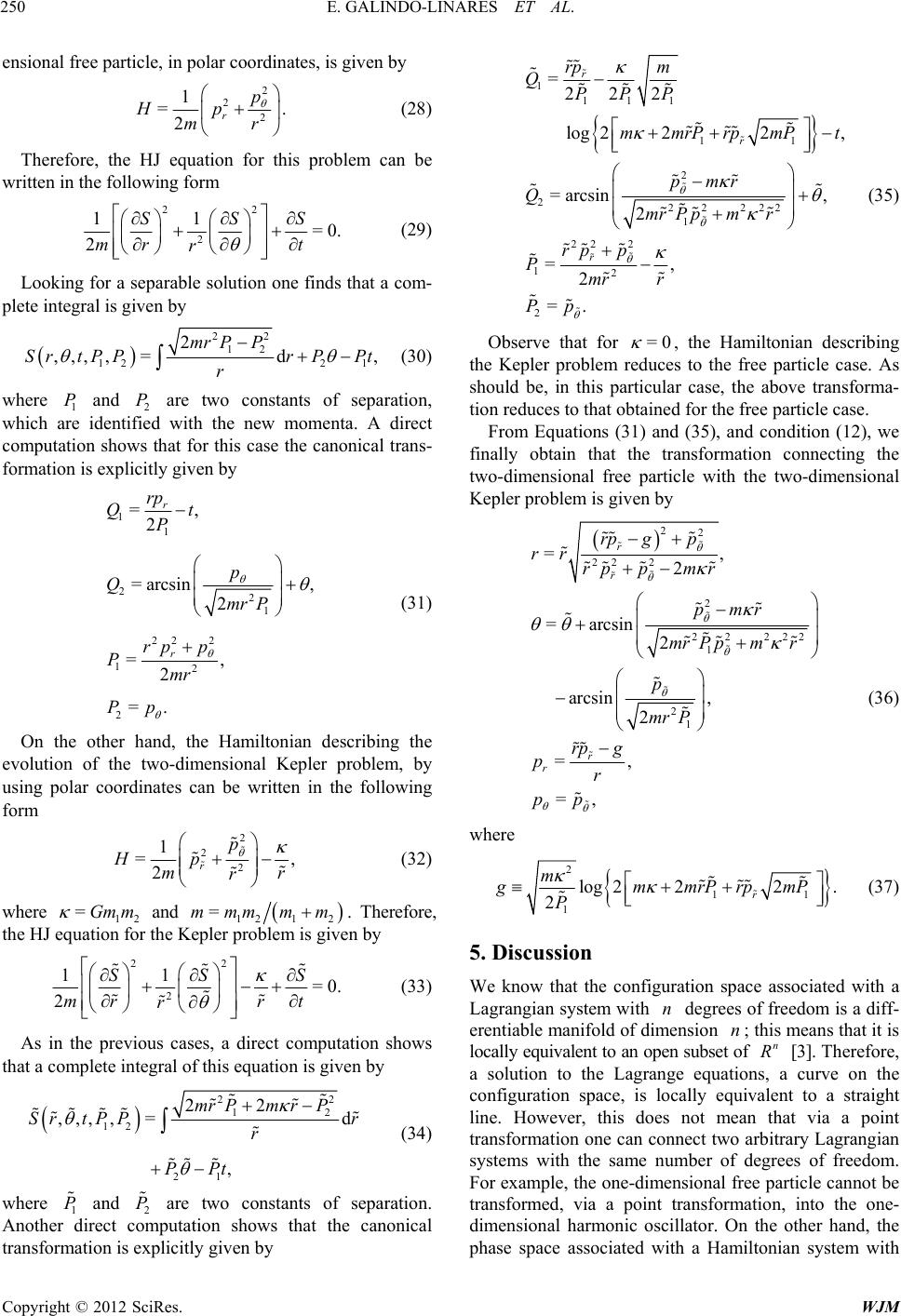 E. GALINDO-LINARES ET AL. 250 ensional free particle, in polar coordinates, is given by 2 2 2 1 = 2r p Hp mr . (28) Therefore, the HJ equation for this problem can be written in the following form 22 2 11 =0. 2 SSS mr t r (29) Looking for a separable solution one finds that a com- plete integral is given by 22 12 122 1 2 ,,,,=d, mr PP SrtPPr PPt r (30) where 1 and 2 are two constants of separation, which are identified with the new momenta. A direct computation shows that for this case the canonical trans- formation is explicitly given by P P 11 221 22 2 12 2 =, 2 =arcsin , 2 =, 2 =. r r rp Qt P p Qmr P rp p Pmr Pp (31) On the other hand, the Hamiltonian describing the evolution of the two-dimensional Kepler problem, by using polar coordinates can be written in the following form 2 22 1 = 2r p Hp mr r , (32) where 12 and =Gmm 12 12 =mmmmm. Therefore, the HJ equation for the Kepler problem is given by 22 2 11 =0. 2 SS S mr rt r (33) As in the previous cases, a direct computation shows that a complete integral of this equation is given by 22 12 12 21 22 ,,, ,=d , mr PmrP Sr tPPr r PPt (34) where 1 and 2 are two constants of separation. Another direct computation shows that the canonical transformation is explicitly given by P P 1 111 11 2 222 222 1 22 2 12 2 =222 log 222, =arcsin , 2 =, 2 =. r r r rp m QPPP mmrP rpmPt pmr QmrP pmr rp p Pr mr Pp % % % % % % % %% % %%% %% %%% %% %% % %% % %%% % % % %% (35) Observe that for =0 , the Hamiltonian describing the Kepler problem reduces to the free particle case. As should be, in this particular case, the above transforma- tion reduces to that obtained for the free particle case. From Equations (31) and (35), and condition (12), we finally obtain that the transformation connecting the two-dimensional free particle with the two-dimensional Kepler probl em is give n by 22 22 2 2 22 222 1 21 =, 2 =arcsin 2 arcsin , 2 =, =, r r r r rp gp rr rp pmr pmr mrP pmr p mr P rp g pr pp % % % % % % % % % %% % % %% %% %% % % %% % % % %% % (36) where 2 1 1 log 222. 2r m gmmrPrp P 1 mP % %% %%% % (37) 5. Discussion We know that the configuration space associated with a Lagrangian system with degrees of freedom is a d iff- erentiable manifold of dimension ; this means that it is locally equivalent to an open subset of [3]. Therefore, a solution to the Lagrange equations, a curve on the configuration space, is locally equivalent to a straight line. However, this does not mean that via a point transformat ion one can connect two arbitrary Lagran gian systems with the same number of degrees of freedom. For example, the one-dimensional free particle cannot be transformed, via a point transformation, into the one- dimensional harmonic oscillator. On the other hand, the phase space associated with a Hamiltonian system with nnn R Copyright © 2012 SciRes. WJM  E. GALINDO-LINARES ET AL. 251 n degrees of freedom is another differentiable manifold, a symplectic manifold, of dimension and thus it is locally equivalent to an open subset of [3]. The canonical transformations, which are defined as those transformations of the phase space such that the Poisson brackets or symplectic structure remains invariant have the property of connectin g two Hamiltonian syste ms with the same number of degrees of freedom. This result is well established and well known. But one of the main contributions of this work was to realize that the very special class of canonical transformations generated via a complete integral of the HJ equation has the property of mapping an entire curve in to a single point. This property was used to show that all the Hamiltonian systems with the same number of degrees of freedom are locally equivalent. Even though all the Hamiltonian systems are locally equivalent to each other, at the Lagrangian level they, in general, give rise to physically nonequivalent Lagrangian systems. For example, as we have shown, the one-dimensional free particle and the one-dimensional harmonic oscillator are locally equivalent in the Hami- ltonian formulation in the sense that there is a canonical transformation that maps one system into the other. But, at the Lagrangian level they cannot be connected via a point transformation; that is, they are two Lagrangian systems describing two different physical situations. Observe that in the Lagrangian formulation the property of invariance in form of Lagrange equations and the fact that the dimension of the configuration space is equal to the number of degrees of freedom of the system, implies that the original Lagrangian system and that obtained under a point transformation describe exactly the same mechanical system. In some sense, in Lagrangian formu- lation, mathematical equivalence implies physical equi- valence. However, in the Hamiltonian formulation it is not true, and it is so, because the dimension of the phase space is two times the number of degrees of freedom of the physical system. As we have remarked, for each Hamiltonian system the extra dimensions added to the configuration space allows to find a co ord ina te sys tem where there is no dynamics. This very important property cannot be found in the Lagrangian formulation. 2n2n R n We finish our work with the following observation: we start with a physical system such that its d ynamics in the Lagrangian formulation is described by the lagrangian function, . Furthermore, we assume that its associated natural Hamiltonian, L , can be computed (the natural Hamiltonian is that obtained via a Legendre transfor- mation). Therefore, at this stage, we have a Hamiltonian system with Hamiltonian function, . Now by perfo- rming a canonical transformation on it we obtain a new Hamiltonian system with Hamiltonian function, . If the natural Lagrangian function, , associated with the new Hamiltonian system is defined, then at the end we have two Lagrangian systems, our observation is that the new Lagrangian system may not describe the original physical system. If the canonical transformation used to obtain the new Hamiltonian system corresponds to a point transformation then both Lagrangian systems des- cribe the same physical situation, but if the used ca- nonical transformation does not come from a point trans- formation, then the two Lagrangian systems describe two different physical situations. We emphasize that there are canonical transformations that give rise to Hamiltonian systems such that its natural Lagrangian is not defined. L 6. Acknowledgements E. Galindo-Linares and E. Navarro-Morales were sup- ported by a CONACyT scholarship. G. Silva-Ortigoza acknowledges financial support from SNI (México). This work has received partial support from VIEP-BUAP. R. Silva-Ortigoza and M. Marciano-Melchor acknowledge financial support from SNI, Secretar de Investigación y Posgrado del IPN (SIP-IPN) and the programs EDI, EDD and COFAA of IPN. REFERENCES [1] L. D. Landau and E. M. Lifshitz, “Mechanics,” 3rd Edi- tion, Butterworth Heinemann, Oxford, 2000. [2] H. Goldstein, C. Poole and J. Safko, “Classical Mechan- ics,” 3rd Edition, Addison Wesley, Boston, 2002. [3] V. I. Arnold, “Mathematical Methods of Classical Me- chanics,” Springer-Verlag, New York, Heidelberg, Berlin, 1984. [4] D. Bergmann and Y. Frishman, “A Relation between the Hydrogen Atom and Multidimensional Harmonic Oscil- lators,” Journal of Mathematical Physics, Vol. 44, 1965, pp. 1855-1856. doi:10.1063/1.1704733 [5] M. Moshinsky, “Canonical Transformations and Quan- tum Mechanics,” Notes of the Latin American School of Physics, University of México, México, 1971. [6] M. Moshinsky, T. H. Seligman and K. B. Wolf, “Ca- nonical Transformations and the Radial Oscillator and Coulomb Problems,” Journal of Mathematical Physics, Vol. 13, No. 6, 1972, pp. 901-907. doi:10.1063/1.1666074 [7] V. I. Arnol’d, “Huygens and Barrow, Newton and Hooke,” Birkhauser-Verlag, Basel, 1990. doi:10.1007/978-3-0348-9129-5 [8] K. Bohlin, “Note sur le Problème des Deux Corps et sur Une Intégration Nouvelle dans le Problème des Trois Co rps,” Bulletin Astronomique, Vol. 28, 1911, pp. 113-119. [9] T. Needham, “Visual Complex Analysis,” Oxford Univer- sity Press, Oxford, 1997. [10] T. Needham, “Newton and the Transmutation of Force,” The American Mathematical Monthly, Vol. 100, No. 2, 1993, p. 119. doi:10.2307/2323768 [11] D. R. Stump, “Arnold’s Transformation an Example of a Generalized Canonical Transformation,” Journal of Mathe- Copyright © 2012 SciRes. WJM  E. GALINDO-LINARES ET AL. Copyright © 2012 SciRes. WJM 252 matical Physics, Vol. 39, No. 7, 1998, pp. 3661-3669. doi:10.1063/1.532458 [12] G. F. T. del Castillo, “On the Connection between the Kepler Problem and the Isotropic Harmonic Oscillator in Classical Mechanics,” Revista Mexicana de Fisica, Vol. 44, No. 4, 1998, pp. 333-338. [13] G. F. T. del Castillo and F. A. de la Cruz, “Connection between the Kepler Problem and the Maxwell Fish-Eye,” Revista Mexicana de Fisica, Vol. 44, No. 6, 1998, pp. 546-549. [14] G. F. T. del Castillo, D. A. R. Álvarez and I. F. Cárcamo, “The Action of Canonical Transformation on Functions Defined on the Configuration Space,” Revista Mexicana de Fisica, Vol. 56, No. 2, 2010, pp. 113-117.
|