 Int. J. Communications, Network and System Sciences, 2012, 5, 671-677 http://dx.doi.org/10.4236/ijcns.2012.510069 Published Online October 2012 (http://www.SciRP.org/journal/ijcns) Structural Properties of Optimal Scheduling Policies for Wireless Data Transmission Nomesh Bolia1, Vidyadhar Kulkarni2 1Department of Mechanical Engineering, Indian Institute of Technology, Delhi, India 2Department of Statistics and Operations Research, University of North Carolina, Chapel Hill, USA Email: nomesh@mech.iitd.ac.in, vkulkarn@email.unc.edu Received August 15, 2012; revised September 12, 2012; accepted October 8, 2012 ABSTRACT We analyze a cell with a fixed number of users in a time period network. The base station schedules to serve at most one user in a given time period based on information about the available data rates and other parameter(s) for all the users in the cell. We consider infinitely backlogged queues and model the system as a Markov Decision Process (MDP) and prove the monotonicity of the optimal policy with respect to the “starvation age” and the available data rate. For this, we consider both the discounted as well as the long-run average criterion. The proofs of the monotonicity proper- ties serve as good illustrations of analyzing MDPs with respect to their optimal solutions. Keywords: MDP; Scheduling; Structural Properties 1. Introduction We consider a fixed set of mobile data users in a wireless cell served by a single base station and focus on the downlink channel. The base station maintains a sepa- rate queue of data for each user. Time is slotted and in each slot (time period in the standard MDP terminology) the base station can transmit data to exactly one user. Let be the channel rate of user during time period , i.e., the amount of data that can be transmitted to user during time period by the base station. We assume that the base station knows at all time periods the vector 12 N. How this information is gathered depends on the system in use. An example of a resource allocation system widely known and used in practice is the CDMA2000 1xEV-DO system [1]. A good description of how this information is generated is also provided in [1]. A good framework for resource allocation and related issues in this (and more general) setting can be found in [2]. N =1,n nn n,,, nnn n RRR R u nn R , ;N =1,2, n u Ru uu There are two objectives to be fulfilled while schedul- ing the data transfer. The first is to obtain a high data transfer rate. This can be achieved by serving a user in period whose channel rate u is the highest, i.e., following a myopic policy. However if we follow the myopic policy, we run the risk of severely starving users whose channel rate is low for a long time. The second objective is to ensure that none of the users is severely starved. Thus these are conflicting objectives and any good algorithm tries to achieve a “good” balance be- tween the two. We have proposed MDP based scheduling policies in [3] to achieve this balance. In this paper, for the sake of completeness we first describe the MDP framework (and our heuristic policies) and then analyze the important monotonicity properties of the (MDP-) op- timal and our recommended policies. Literature Survey This problem of scheduling users for data transmission in a wireless cell has been considered in the literature mostly in the last decade and a half. One of the most widely used algorithms that takes advantage of multiuser diversity (users having different and time-varying rates at which they can be served data) while at the same time being fair to all users is the Proportional Fair Algorithm (PFA) of Tse [4]. When each user always has data to be served waiting at the base station (infinitely backlogged queues), the PFA performs well and makes good use of the multiuser diversity. However, it has been proven to be unstable when data isn’t always available to be served to each user, and instead, there is external data arrival [5]. Most of the algorithms in this setting are not necessarily outcomes of any optimization framework. In our earlier publication [3], we take a novel approach to solving this problem. This approach develops the scheduling algo- rithm as an outcome of a systematic optimization frame- work. Therefore, Bolia and Kulkarni [3] develop MDP and policy improvement based scheduling policies. These policies are easy to implement, and shown to per- C opyright © 2012 SciRes. IJCNS  N. BOLIA, V. KULKARNI 672 form better [3] than existing policies. However, while our recommended policies despite being sub-optimal exhibit better results than existing po- licies [3], our past work lacks any results about structural properties of both the recommended as well as the opti- mal policies. We believe it is important to establish some such properties to either gain further insight into the problem. Therefore, in this correspondence we prove some mono tonicity properties of the optimal policies and the policies proposed in [3]. We first define and describe these monotonicity properties in the paper. Our contribu- tions are two fold: A rigorous analysis of these properties along with the observation that our recommended policy in [3] is also monotone (thus being in line with the opti- mal policy at least with respect to some basic properties) and an illustration of analysis of optimal policies in the MDP framework. These ideas can serve as a good start- ing point and provide broad guidelines to analyze struc- tural properties of MDPs. The rest of the article is organized as follows: Section 2 describes the model and index policy and Section 3 proves monotonicity of the optimal policy in this setting. Section 3.3 extends the results for these properties to the long-run average criterion. We conclude the paper with remarks on possible extensions in Section 4. 2. The Model In this section, for the sake of completeness, we start with a description of the stochastic model [3] for the multidimensional stochastic process that represents the channel rates of all users in the cell. Let u ,1 n Rn n be the channel state of user u at time . This represents various factors such as the position of the user in the cell, the propagation conditions, etc. and deter- mines the channel rate of user u as described below. We assume that is an irreducible Discrete Time Markov chain (DTMC) on state space n =1,2, n u R ,1 n u Xn , , uu ij =11 with Transition Probability Matrix (TPM) . Note that the TPM can in general = u Pu p be different for different users. Further, as indicated in [1], a set of fixed data rates is what is available to users in an actual system. For each , let k be the fixed data rate (or channel rate) associated with state of the DTMC u. Thus, when u =1,2, ,uN k ,1 n Xn n r = k :Rn , the user can receive data from the base station at rate if it is chosen to be served. Thus is a Markov Chain with state space u = uk r n 1 R n u 12 , i.e., the vector of all fixed data rates. We assume, without loss of generality, that 12 =,rr,r, M r rr r. Let 1N =,, nn XX n X be the state vector of all the users. We assume the users behave independently of each other and that each user has ample data to ber served. This setting where each user always has ample data to be served is referred to as the “infi- nitely backlogged queues setting”. Since each component of ,1 n Xn is an independent DTMC on , it is clear that ,1 n XnN n Yu nu 1n itself is a DTMC on . Let u be the “starvation age” (or simply “age”) of the user at time , defined as the time elapsed (in number of periods) since the user was served most recently. Thus, the age of the user is zero at time if it is served in the time period. Furthermore, for , if the user was served in time period and it is not served for the next time periods, its age at time th n 1mn m nm is 1m . Let 1N YY be the age vector (vector of ages of all users) at time . The base station serves exactly one user in each time period. Let =,, nn n Y n vn th n 11if , =0if =. n u n u Yuvn Yuvn n , nnN N be the user served in the time period. The age process evolves according to (1) The “state of the system” at time is given by YZ =0,1,2,Z 2N , nn , where . The “state” is thus a vector of components and we assume that it is known at the base station in each time period. After observing Y the base station decides to serve one of the users in the time period . We need a reward structure in order to make this decision optimally. We describe such a structure below. If we serve user in the time period, we earn a reward equal to n u u Nn u th n = n Rr Dy ly n for this user and none for the others. In addition, there is a cost of l if user of age is not served in period . This cost corresponds to the penalty incurred due to “starvation” of the user(s) not served in a given time period. Clearly, we can assume 0=0Du n . nn ull lu RDY l since there is no starvation at age zero. Thus the net reward of serving user at time is (2) We assume that there is no cost in switching from one user to another from period to period. This is not entirely true in practice, but including switching costs in the model will make the analysis intractable. For conven- ience we use the notation . The pro- = nn ull lu WDY blem of scheduling a user in a given time period can now be formulated as a Markov Decision Process (MDP). The decision epochs are 1, 2,n , nn . The state at time is Y with Markovian evolution as described above. The action space in every state is 1, 2,, N u u , nn where action corresponds to serving the user . The reward in state Y u nn uu RWu t corresponding to action is . For the sake of notational convenience, let and u Wt be defined as follows: Copyright © 2012 SciRes. IJCNS  N. BOLIA, V. KULKARNI 673 11 =1, ,1,0, uuu tt tt 1 1, ,1 N t (3) and, = . ull lu Dt ()Wt (4) Let be the discounting rate for the MDP [6]. Then, the standard Bellman equation for the discounted reward model is =1,2, , ,= max u iu uN VitrW t , , u hit (5) where , Nij j pVjt ,deci tA ,=hit (6) Let be the optimal decision made (i.e., the user served) in state ,it , u hit . Then, =1,2, , ,=arg max u uN iu deci trWt , u uk hit k , . Further, let =1,2, , ,=arg max u ki uN deci trWt th (7) be the optimal decision at the step of the value it- eration scheme given by (8). We use the following notation: For any real valued function it NN defined on , t denotes that decreases in every component of . t u 3. Monotonicity of Optimal Policy Although solving Equation (5) to optimality is infeasible, we can derive some important characteristics of the op- timal policy. In this section, we consider two monotonic- ity properties of the optimal policy. We first consider monotonicity in age. 3.1. Monotonicity in Age The intuition behind monotonicity is as follows. The pen- alty accrued for each user in a given time period is an increasing function of its current age. Hence we expect the propensity of the optimal policy serving any given user to increase with its age, i.e., if the optimal policy serves a user in the state ,it u, it will serve user in state ,iteN th ,Vitt 1=1,2, , ,=, , max 0. u u kiuk uN VitrWt hit k u e as well, where u denotes an - dimensional vector with the u component 1 and all other components 0. Theorem 3.2 states and proves this monotonicity prop- erty of the optimal policy for discounted reward. Then we show that standard MDP theory [6] implies the result holds in the case of long-run average reward as well. We will need the following result to prove theorem 3.2. Theorem 3.1 . Proof. The standard value iteration equations of (5) are given by (8) where ,= ,, kijk j hitpV jt (9) 0,=0Vit . We have and ,=,,,. lim NN k kVitVititZ (10) We will prove ,t tk k Vi using induction on . Then the theorem follows from the above equation. ,t t=0k k Vi holds at since Note that ,=0Vit 0. Assume ,t t0 k k Vi for some . We prove 1, k Vitt . It is enough to prove that 111 ,,0, kk VitVite kk ht (11) since the proof for all components other than 1 follows similarly. Note that Vt . We consider four cases: Case 1: ,=1 k deci t 1 ,=1 k deci te and . From (8), 1 1 111 1 1 1 11 1 ,, =(), ,0, kk ik ik VitVite rWt hit r Wtehite (12) since =v Wte Wt = vv v te t vv and using Equa- tions (3) and (4). Case 2: ,=1deci t ,=1 k deci teu k and 1. From (8), and using 1u Wte Wt 11 = uu tet eu and , we have 1 1 1 111 1 1 11 1 1 1 1 1 ,, =, , ,, ,,0. u u u kk ik u iu k iiu u kk iiu u kk VitVite rWt hit r Wtehite rr WtWt hithite rr WtWt hit hit ht ,=1decit (13) The second inequality holds because k and the last inequality holds because . k Case 3: ,= 1 k deci tu and From (8), 1 ,=. k deci teu Copyright © 2012 SciRes. IJCNS  N. BOLIA, V. KULKARNI 674 11 1 ,, =, ,, u u kk iuk iu uu uu kk VitVite rWthi r Wteh Wte Wt hit hit 1 11 1 , 0, u u k t ite e ,=i t 1 ,=.i teu 1 11 1 , ] u v k u u t ite Wt e Wt ,=deci tu ,tt kt k , = v i tev ,, . u ituA (, )= i tev v 0, v v u vv Wte te =v vv e (14) using the same arguments as in Case 2. Case 4: k and k From (8), and using and , we have 1udec 1vv Wte Wt (,)Vite dec 1 = vv tete (,Vi 1 t 11 =, (, ) , [] ,, 0. u v uv kk iuk iv ii v uv kk ii v uv uv kk rW t hi r Wteh rr Wt hit hit rr Wt hithit (15) The last inequality holds because . k Clearly, Cases 1 - 4 are exhaustive and thus Equations (12) through (15) prove that 1k Vi , thus completing our induction argument. Hence V for all . This completes the proof. Now we move on to the main theorem of this section that says that the decision to serve a user in any time period is monotone in age. Theorem 3.2 . ,=deci tvdec ,=deci tvProof. Since we have, () , v u v iv iu t hit rWth rW (16) To prove , we need to prove dec rr ,, vu iiu v v Wte hite hi (17) which follows from (16) (and tt ), and the results that = vvv e WtWt , uv e Wt <, u hit v u [using Equation (4)] and [using theorem 3.1 and Equation (6)]. Wt , u v ehi t This theorem implies that if it is optimal to serve a given user, say , in a given state ,it v of the system, it is optimal to serve the same user when everything is identical except the age of the same user () increases by one. Thus, everything else remaining constant, the opti- mal policy is monotone in the age of the users, a result we expect intuitively for any reasonable scheduling pol- icy, but now proved rigorously for the optimal policy. Similarly, the rest of the theorems in the paper provide rigor to intuitively expected monotonocity in different settings. 3.2. Monotonicity in Rate The MDP model has been formulated to maximize the infinite horizon expected total discounted net reward. The net reward over one time period in a given state ,it v equals the data rate of the user that is chosen to serve minus the penalty accrued by all other users. We expect the optimal policy to be monotone in the rate that can be potentially available to the users. In particular, we expect that if the optimal policy serves user in state ,it v , then it will serve in state ,iet ,1 n Xn v as well. We prove this in theorem 3.3. The proof of theorem 3.3 is similar (but more tedious) to the proof of theorem 3.2. However, it needs the additional condition of stochastic monotonicity of DTMCs, see [7]. Theorem 3.3 If the Markov chain is stochastically monotone, then ,= ,= v deci tvdecietv . (18) ,=decitv we have, Proof. Since , ,, . v u v iv u iu rWthit rWthituA (19) To prove ,=dec itv ,,0. vv vu uv ie ie vu vv rr WtWt hiethi et , we need to prove (20) To establish this, we can first prove ,,,, vuvu vv Vi etVietVitVit (21) by considering the set of exhaustive cases similar to the proof of theorem 3.1. Stochastic monotonicity then im- plies ,,,,, vuvu vv hie thie thithit (22) which yields 20, as required. 3.3. Long-Run Average Reward Criterion In this section we extend the results of Section 3 to the long-run average reward criterion. As is well known, the objective in long-run average reward models is to maxi- mize the long-run average reward, instead of the ex- pected total discounted reward as considered in (5). If Copyright © 2012 SciRes. IJCNS 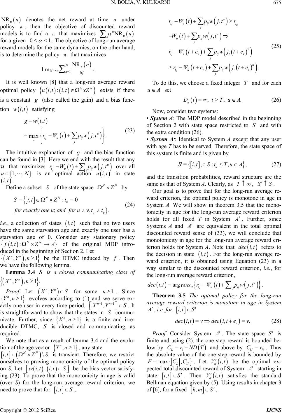 N. BOLIA, V. KULKARNI 675 NR nn π π π denotes the net reward at time under policy , then the objective of discounted reward models is to find a that maximizes NR nn 0<1 π n for a given . The objective of long-run average reward models for the same dynamics, on the other hand, is to determine the policy that maximizes π π =1 NR N n n N ,NN t xZ limN . It is well known [8] that a long-run average reward optimal policy exists if there is a constant ,:uit i (also called the gain) and a bias func- tion satisfying ,wit , = max u iu uj gwit rWt , . u ij pwjt (23) The intuitive explanation of and the bias function can be found in [3]. Here we end with the result that any that maximizes ij j u over all is an optimal action u ,u pwjt u iu rWt 1,, N ,tui in state ,it NN . Define a subset of the state space S by =, := NN u SitZt 0 ;,, uv orexactlyone uandforu v tt ,it (24) i.e., a collection of states such that no two users have the same starvation age and exactly one user has a starvation age of 0. Consider any stationary policy ,:NN it ,, nn XY Z 1n A of the original MDP intro- duced in the beginning of Section 2. Let be the DTMC induced by . Then we have the following lemma. Lemma 3.4 is a closed communicating class of S ,,1 nn XY n , nn . Proof. Let Y1n 11 , nn S for some . Since evolves according to (1) and we serve ex- actly one user in every time period, ,1 n Yn YS . It is straightforward to show that the states in commu- nicate. Further, since is a finite and irre- ducible DTMC, is closed and communicating, as required. S ,1 n Yn n,1Xn S We note that as a result of lemma 3.4 and the evolu- tion of the age vector , any state , NN Z ,:wit \S ,it S it is transient. Therefore, we restrict ourselves to proving monotonicity of the optimal policy on S. Let be the bias vector satisfy- ing (23). To prove that the monotonicity in age is valid (over S) for the long-run average reward criterion, we need to prove that for ,it S, , , , ,. v v u v iv iji u j u uij j v iv vijv j u iu vijv j rWtpwjt r Wt pwjt rWte pwjte rWtepwjte T uA (25) To do this, we choose a fixed integer and for each set =,>, u Dtt Tu A. S (26) Now, consider two systems: • System A: The MDP model described in the beginning of Section 2 with state space restricted to and with the extra condition (26). • System A׳: Identical to System A except that any user with age T has to be served. Therefore, the state space of this system is finite and is given by '=,,:,, u SitStTuA T SS (27) and the transition probabilities, reward structure are the same as that of System A. Clearly, as , . Our goal is to prove that for the long-run average re- ward criterion, the optimal policy is monotone in age in System A. We will show in theorem 3.5 that the mono- tonicity in age for the long-run average reward criterion holds for all fixed T in System . Further, since Systems A and are equivalent in the total optimal discounted reward sense of (33), we will conclude that monotonicity in age for the long-run average reward cri- terion holds for System A. Note that refers to the decision in state ,deci t ,it . For the long-run average re- ward criterion, it is obtained using Equation (23) in a way similar to the discounted reward criterion, i.e., for the long-run average reward criterion, ,=arg , max u u uiu ij j deci trWtp wj t . Theorem 3.5 The optimal policy for the long-run average reward criterion is monotone in age in System , i.e. for ,it S ,=, = v deci tvdecitev. (28) Proof. Consider System S. The state space is finite and using (2), the one step reward is bounded be- low by =CrNDT=Cr 1L and above by UN . Thus the absolute value of the one step reward is bounded by =max , LU CC ,t . Let Vi be the optimal ex- pected total discounted reward of System starting in state ,it S . Then Vi satisfies the standard Bellman equation given by (5). Using results in chapter 3 of [6], for a fixed ,t ,km S , Copyright © 2012 SciRes. IJCNS 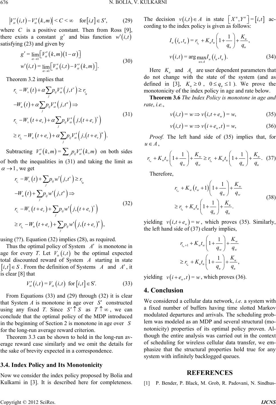 N. BOLIA, V. KULKARNI 676 ,vit A ,,<<Vit VkmC ,=, nn for,,it S C (29) where is a positive constant. Then from Ross [9], there exists a constant and bias function ,wit 1 , .Vkm , ,. i u v v u v r jte jte , ij jpVkm 1 satisfying (23) and given by 1 1 =, lim ,= , lim gVkm witV it (30) Theorem 3.2 implies that , , v v u v iv ij j u uij j iv vij j iu vij j rWtpVjt WtpV jt rWte pV rWtepV (31) Subtracting on both sides ,=Vkm of both the inequalities in (31) and taking the limit as , ,, i u v v u v r jte jte , we get , , v v u v iv ij j u uij j iv vij j iu vij j rWtpwjt Wt pwjt rWte pw rWtepw (32) using (??). Equation (32) implies (28), as required. Thus the optimal policy of System ,t is monotone in age for every T. Let be the optimal expected total discounted reward of System Vi starting in state ,it S. From the definition of Systems and , it is clear [8] that ,= ,V itV it for,Sit S S . (33) From Equations (33) and (29) through (32) it is clear that System A is monotone in age over constructed using any fixed T. Since S as , we can conclude that the optimal policy of the MDP introduced in the beginning of Section 2 is monotone in age over for the long-run average reward criterion. T S Theorem 3.3 can be shown to hold in the long-run av- erage reward case similarly and we omit the details for the sake of brevity expected in a correspondence. 3.4. Index Policy and Its Monotonicity Now we consider the index policy proposed by Bolia and Kulkarni in [3]. It is described here for completeness. The decision in state Yit ac- cording to the index policy is given as follows: 1 ,= 1, u u uuu iuu uu IitrKtqq ,=arg, . max uuu uA vitIit (34) Here u and u are user dependent parameters that do not change with the state of the system (and as defined in [3], u, u). We prove the monotonicity of the index policy in age and rate below. 0K01q Theorem 3.6 The Index Policy is monotone in age and rate, i.e., ,=,=, w vitwvitew (35) ,= ,=, w vit wviet w uA (36) Proof. The left hand side of (35) implies that, for , 11 11 wu wu iww iuu ww uu . K rK t rKt qq qq (37) Therefore, 1 11 1 1. w u w iww ww u iuu uu rKt qq K rKt qq (38) yielding ,=viteww, which proves (35). Similarly, the left hand side of (37) clearly implies, 1 1 1 1 1, w u w iww ww u iuu uu rKtqq rKt qq ,= w vie tw, which proves (36). yielding 4. Conclusion We considered a cellular data network, i.e. a system with a fixed number of buffers having time slotted Markov modulated departures and arrivals. The scheduling prob- lem was modeled as an MDP and several structural (mo- notonicity) properties of its optimal policy proven. Al- though the entire analysis was carried out in the context of scheduling for wireless cellular data transfer, we em- phasize that the structural properties hold true for any system with infinitely backlogged queues. REFERENCES [1] P. Bender, P. Black, M. Grob, R. Padovani, N. Sindhus- Copyright © 2012 SciRes. IJCNS  N. BOLIA, V. KULKARNI Copyright © 2012 SciRes. IJCNS 677 hayana and A. Viterbi, “CDMA/HDR: A Bandwidth Ef- ficient High Speed Wireless Data Service for Nomadic Users,” IEEE Communications Magazine, Vol. 38, No. 7, 2000, pp. 70-77. doi:10.1109/35.852034 [2] L. Georgiadis, M. J. Neely and L. Tassiulas, “Resource Allocation and Cross-Layer Control in Wireless Net- works,” Foundations and Trends in Networking, Vol. 1, No. 1, 2006, pp. 1-144. doi:10.1561/1300000001 [3] N. Bolia and V. Kulkarni, “Index Policies for Resource Allocation in Wireless Networks,” IEEE Transactions on Vehicular Technology, Vol. 58, No. 4, 2009, pp. 1823- 1835. doi:10.1109/TVT.2008.2005101 [4] D. Tse, “Multiuser Diversity in Wireless Networks,” 2011. http://www.eecs.berkeley.edu/~dtse/stanford416.ps [5] M. Andrews, “Instability of the Proportional Fair Sched- uling Algorithm for HDR,” IEEE Transactions on Wire- less Communications, Vol. 3, No. 5, 2002, p. 2004. [6] Q. Hu and W. Yue, “Markov Decision Processes with Their Applications,” Springer, New York, 2008. [7] I. Kadi, N. Pekergin and J. M. Vincent, “Analytical and Stochastic Modeling Techniques and Applications,” Spri- nger, New York, 2009. [8] M. Puterman, “Markov Decision Processes: Discrete Sto- chastic Dynamic Programming,” John Wiley & Sons, Inc, New York, 1994. [9] S. M. Ross, “Introduction to Stochastic Dynamic Pro- gramming,” Academic Press, Inc., New York, 1983.
|