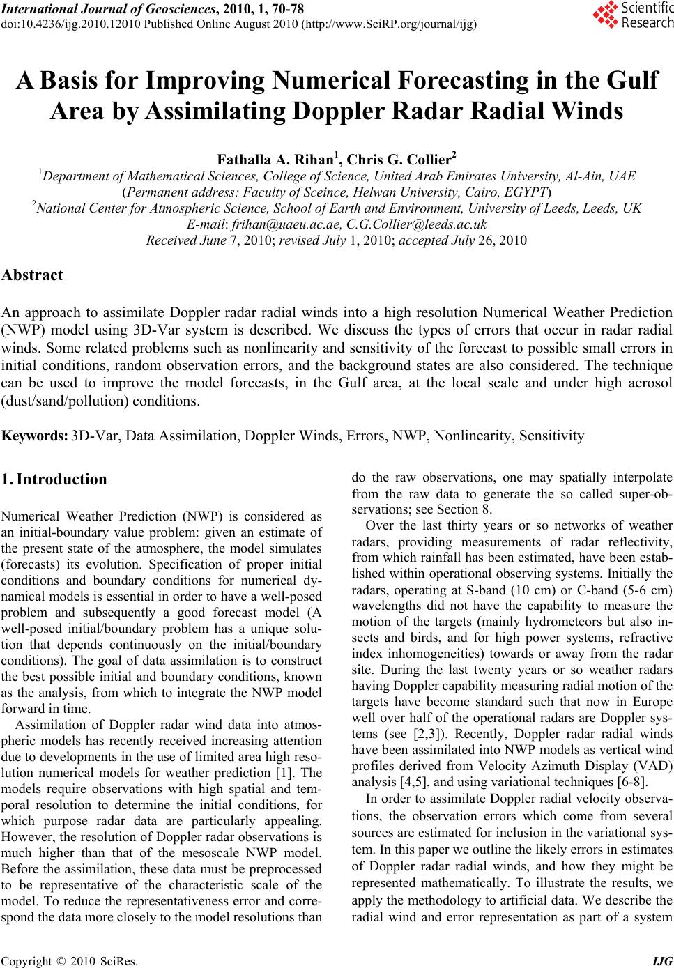International Journal of Geosciences, 2010, 1, 70-78
doi:10.4236/ijg.2010.12010 Published Online August 2010 (http://www.SciRP.org/journal/ijg)
A Basis for Improving Numerical Forecasting in the Gulf
Area by Assimilating Doppler Radar Radial Winds
Fathalla A. Rihan1, Chris G. Collier2
1Department of Mathematical Sciences, College of Science, United Arab Emirates University, Al-Ain, UAE
(Permanent address: Faculty of Sceince, Helwan University, Cairo, EGYPT)
2National Center for Atmospheric Science, School of Earth and Environment, University of Leeds,
Leeds, UK
Received June 7, 2010; revised July 1, 2010; accepted July 26, 2010
Abstract
An approach to assimilate Doppler radar radial winds into a high resolution Numerical Weather Prediction
(NWP) model using 3D-Var system is described. We discuss the types of errors that occur in radar radial
winds. Some related problems such as nonlinearity and sensitivity of the forecast to possible small errors in
initial conditions, random observation errors, and the background states are also considered. The technique
can be used to improve the model forecasts, in the Gulf area, at the local scale and under high aerosol
(dust/sand/pollution) conditions.
Keywords: 3D-Var, Data Assimilation, Doppler Winds, Errors, NWP, Nonlinearity, Sensitivity
1. Introduction
Numerical Weather Prediction (NWP) is considered as
an initial-boundary value problem: given an estimate of
the present state of the atmosphere, the model simulates
(forecasts) its evolution. Specification of proper initial
conditions and boundary conditions for numerical dy-
namical models is essential in order to have a well-posed
problem and subsequently a good forecast model (A
well-posed initial/boundary problem has a unique solu-
tion that depends continuously on the initial/boundary
conditions). The goal of data assimilation is to construct
the best possible initial and boundary conditions, known
as the analysis, from which to integrate the NWP model
forward in time.
Assimilation of Doppler radar wind data into atmos-
pheric models has recently received increasing attention
due to developments in the use of limited area high reso-
lution numerical models for weather prediction [1]. The
models require observations with high spatial and tem-
poral resolution to determine the initial conditions, for
which purpose radar data are particularly appealing.
However, the resolution of Doppler radar observations is
much higher than that of the mesoscale NWP model.
Before the assimilation, these data must be preprocessed
to be representative of the characteristic scale of the
model. To reduce the representativeness error and corre-
spond the data more closely to the model resolutions than
do the raw observations, one may spatially interpolate
from the raw data to generate the so called super-ob-
servations; see Section 8.
Over the last thirty years or so networks of weather
radars, providing measurements of radar reflectivity,
from which rainfall has been estimated, have been estab-
lished within operational observing systems. Initially the
radars, operating at S-band (10 cm) or C-band (5-6 cm)
wavelengths did not have the capability to measure the
motion of the targets (mainly hydrometeors but also in-
sects and birds, and for high power systems, refractive
index inhomogeneities) towards or away from the radar
site. During the last twenty years or so weather radars
having Doppler capability measuring radial motion of the
targets have become standard such that now in Europe
well over half of the operational radars are Doppler sys-
tems (see [2,3]). Recently, Doppler radar radial winds
have been assimilated into NWP models as vertical wind
profiles derived from Velocity Azimuth Display (VAD)
analysis [4,5], and using variational techniques [6-8].
In order to assimilate Doppler radial velocity observa-
tions, the observation errors which come from several
sources are estimated for inclusion in the variational sys-
tem. In this paper we outline the likely errors in estimates
of Doppler radar radial winds, and how they might be
represented mathematically. To illustrate the results, we
apply the methodology to artificial data. We describe the
radial wind and error representation as part of a system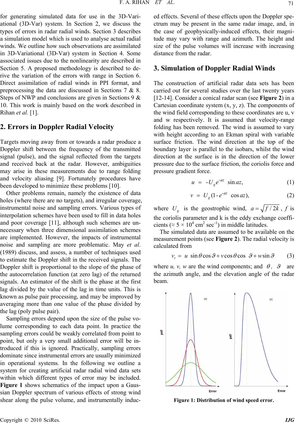

F. A. RIHAN ET AL.
71
for generating simulated data for use in the 3D-Vari-
ational (3D-Var) system. In Section 2, we discuss the
types of errors in radar radial winds. Section 3 describes
a simulation model which is used to analyse actual radial
winds. We outline how such observations are assimilated
in 3D-Variational (3D-Var) system in Section 4. Some
associated issues due to the nonlinearity are described in
Section 5. A proposed methodology is described to de-
rive the variation of the errors with range in Section 6.
Direct assimilation of radial winds in PPI format, and
preprocessing the data are discussed in Sections 7 & 8.
Steps of NWP and conclusions are given in Sections 9 &
10. This work is mainly based on the work described in
Rihan et al. [1].
2. Errors in Doppler Radial Velocity
Targets moving away from or towards a radar produce a
Doppler shift between the frequency of the transmitted
signal (pulse), and the signal reflected from the targets
and received back at the radar. However, ambiguities
may arise in these measurements due to range folding
and velocity aliasing [9]. Fortunately procedures have
been developed to minimize these problems [10].
Other problems remain, namely the existence of data
holes (where there are no targets), and irregular coverage,
instrumental noise and sampling errors. Various types of
interpolation schemes have been used to fill in data holes
and poor coverage [11], although such schemes are un-
necessary when three dimensional assimilation schemes
are implemented. However, the impacts of instrumental
noise and sampling are more problematic. May et al.
(1989) discuss, and assess, a number of techniques used
to estimate the Doppler shift in the received signals. The
Doppler shift is proportional to the slope of the phase of
the autocorrelation function (at zero lag) of the returned
signals. An estimator of the shift is the phase at the first
lag divided by the value of the lag in time units. This is
known as pulse pair processing, and may be improved by
averaging more than one value of the phase divided by
the lag (poly pulse pair).
Sampling errors depend upon the size of the pulse vo-
lume corresponding to each data point. In practice the
sampling errors could be weakly correlated from point to
point, but only a very small additional error will be in-
troduced if this is ignored. Practically, sampling errors
dominate since instrumental errors are usually minimized
in operational systems. In the following we outline a
system for creating artificial radar radial wind data sets
within which different types of error may be included.
Figure 1 shows schematics of the impact upon a Gaus-
sian Doppler spectrum of various effects of strong wind
shear along the pulse volume, and instrumentally induc-
ed effects. Several of these effects upon the Doppler spe-
ctrum may be present in the same radar image, and, in
the case of geophysically-induced effects, their magni-
tude may vary with range and azimuth. The height and
size of the pulse volumes will increase with increasing
distance from the radar.
3. Simulation of Doppler Radial Winds
The construction of artificial radar data sets has been
carried out for several studies over the last twenty years
[12-14]. Consider a conical radar scan (see Figure 2) in a
Cartesian coordinate system (x, y, z). The components of
the wind field corresponding to these coordinates are u, v
and w respectively. It is assumed that velocity-range
folding has been removed. The wind is assumed to vary
with height according to an Ekman spiral with variable
surface friction. The wind direction at the top of the
boundary layer is parallel to the isobars, whilst the wind
direction at the surface is in the direction of the lower
pressure due to the surface friction, the coriolis force and
pressure gradient force.
-
- sin,
g
az
uUeaz (1)
-
(1- cos),
g
az
vU eaz (2)
where
g
U is the geostrophic wind, /2afk, f is
the coriolis parameter and k is the eddy exchange coeffi-
cients (≈ 5 × 104 cm2 sec-1) in middle latitudes.
The simulated data are assumed to be available on the
measurement points (see Figure 2). The radial velocity is
calculated from
sincoscoscos sin
r
vu vw



 (3)
where u, v, w are the wind components; and

,

are
the azimuth angle, and the elevation angle of the radar
beam.
Figure 1: Distribution of wind speed error.

F. A. RIHAN ET AL.
72
Figure 2. Geometry for scan of velocities on a Velocity Azi-
muth Display (VAD) circle (top) and the variation of the
radial.
At each measurement point a Gaussian (or a modifica-
tion of a Gaussian) distribution is introduced, the magni-
tude and spatial variation of which may represent the
different error types shown in Figure 1. Examples of the
type of artificial radial velocity field produced using
Formula (3) are displayed in Figure 3 (top). Such data
can be used to test the representation of the errors in the
Doppler radial winds, and variational analysis schemes.
Air movement is 3-dimensional and varies over time
and space. However, Doppler radar allows the measure-
ment of only one (radial) component of the velocity of
the targets at a specific range and azimuth. Since we only
take the data from single radar in the present study rather
than simultaneous measurements with three Doppler
radars, we are forced to make a simplifying assumption
to the structure of the observed wind field during the
creation of Doppler products.
The simplest case is to consider a horizontally uniform
wind field for both, horizontal and vertical (precipitation
fall velocity) components. In such a case, if we make
measurements of the velocity along circles centred at the
radar by azimuthal scanning at a constant elevation angle
(PPI), we get, for a constant distance from the radar, a
sinusoidal dependency of the measured radial velocity on
the azimuthal angle. Assuming that the horizontal wind
velocity vh and hydrometeor fall speed w are uniform
over the area being observed, then the mean Doppler
velocity vr varied sinusoidally with maxima and minima
occurring when the beam azimuth passes the upwind (θ
= 0) and downwind (θ = π) directions, that is when
r1 h
r1 h
= cos + sin , when = 0(4)
= - cos + sin , when =
vv w
vv w





Hence
12 12
=, (5)
2cos 2sin
rr rr
h
vv vv
vw



Then the horizontal divergence is given by the formula
2
0
12tan
div, (6)
cos
hr
w
vvd
RR






where R is the radius of the radar sampling circle at
height l. However, Equation (6) is only valid for low ele-
vation angles.
Using Formula (3) to derive the wind velocity, we
compare a plot derived from Figure 3 (top) with a per-
fect sine wave displayed in Figure 3 (bottom). The im-
pact of the simulated errors is to cause the differences
between the data (dots) and the no error sine curve (solid
line) shown. It is possible to use the simulator to investi-
gate, in more detail, the impact of various errors on the
radial winds. This is the subject of continuing study.
4. 3D-Var Data Assimilation
3D-Var systems use an incremental formulation (for a
review see, for example, [6]). Under the assumption that
the background and observation errors are Gaussian,
random and independent of each other, the optimal esti-
mate of the Cartesian wind ab
X
XX

 in the
analysis space is given by the incremental cost function,
1
-1
1
[]
2
1[-][-], (7)
2
T
T
bb
JXXB X
HXYHXE HXYHX





where ab
X
XX


 is the state vector of the analysis
increments (the estimated radial winds is given by
b
a
X
X  HH
, b
X
the state variable of the background
Cartesian winds, and Y denotes the observed radial
winds in the observation space. H is the nonlinear ob-
servation operator that relates the model variables to the
observation variable and a transformation between the
different grid meshes, and
H
is the linear observation
operator with elements /j
hX 
ij i
H. Some construc-
tions of the background and observation error covariance

F. A. RIHAN ET AL.
73
matrices B and E are given in [15]. Miller and Sun [16],
and Xu and Gong [14] assumed that the observation error
covariance matrix E is diagonal with constant diagonal
elements given by the estimated observation error, which
was taken as 1 m/s for typical radar observations. In the
next Section, we provide a different approach to the rep-
resentation of the error of observed radial winds.
To avoid the computationally overwhelming problem
of inverting the covariance matrix B in the minimization
of the cost function (7), and to accelerate the conver-
gence of the minimization algorithm, a pre-conditioning
of the minimization problem is needed [15]. This can be
achieved by defining a variable U to be applied to the
assimilation increment
X

(UX

X) such that it
transforms the forecast error

in the model space into

 a variable of an identity covariance matrix (i.e.,
, I
T
 
 , where .,. is an inner product). This
change of variable can be written as 1 U



. Thus
11
,,, .(8)
TT T
BU UorBUU  

 

Figure 3. Artificial radial velocity with Gaussian noise.
This leads to a new representation of the incremental
cost function of the form
1-1
1
11
[][ -]
22
[- ].(9)
TT
b
b
JHUYXE
HUY X


 

XXXXH
XH
With this cost function, no inversion of B is needed.
The control variables X are velocity potential, stream
function, unbalanced pressure and relative humidity.
Here, we assume that the matrix E includes the errors
from the observations (original measurements), observa-
tion operator, and super-obbing procedure1. The 3D-Var
analysis is then performed using continuous cycling pro-
cedure. The length of the assimilation window in each
analysis is determined according to the model resolution.
In each analysis cycle, the optimal analysis is obtained
by minimizing the cost function (9) using iterative pro-
cedure.
The matrix 1 U

in (9) may be realized as
1
UDF
 (10)
where D is a diagonal matrix of standard deviation of the
background error specified by the error estimation of
numerical experiments, and F is the square root of a ma-
trix whose diagonal elements are equal to one, and off-
diagonal elements are the background error correlation
coefficients. In practical data assimilation for NWP, the
full matrix
F
is too large to compute explicitly or store
into computer memory. Assumptions and approxima-
tions are made such that the effect of
F
on the control
variable X in Equation (9) is achieved through the use
of equivalent spatial filter. Following the work of Purser
and McQuigg [17], Lorenc [18], and Hayden and Purser
[19], the effect of F using a recursive filter is defined by
1i
1i
= +(+1)for = 1,2,...,
Ζ= + (+1); for = ,-1,..., 1;
ii
ii
Xi n
Yinn




 

 (11)
where i
X
is the initial value at grid point i, i

(1,...,in

) is the value after filtering, and i

is the
initial value after one pass of the filter in each direction.

is the filter coefficients given in [15] by
22
1(2),2/(4)Nx L    (12)
where L is the horizontal correlation scale,
x

is the
grid spacing, and N is the number of filter passes to be
applied. This is a first-order recursive filter, applied in
both directions to ensure zero phase change. Multipass
filters (N greater than unity) are built up by repeating
application of (11). This filter can be constructed in all
1Super-obbing procedure is a technique to combine (re-scale) the radar
observations, using statistical interpolation, at a larger spatial scale
which is compatible with the model.

F. A. RIHAN ET AL.
74
three directions. We next provide an approach to esti-
mating the error covariance of radial velocity observa-
tions can be constructed in all three directions up by re-
peating application of (11). This filter can be constructed
in all three directions.
We next provide some related issues due to nonlinear-
ity of the dynamic system.
5. Nonlinearity of the Atmospheric
Dynamics
In general, forecast skill increases not only by increasing
model resolution, but also by improving the numerical
models and the method of solution. However, even if we
had a forecast model that represented atmosphere proc-
esses perfectly, we would never be able to predict the
state of atmosphere accurately for long lead times. A
chaotic behavior occurs (and leads to an unpredictable
long-term evolution) when solving deterministic, non-
linear, dynamical systems that exhibit sensitivity to ini-
tial conditions. This occurs, because the nonlinear dy-
namical systems that describe the atmospheric behaviour
are sensitive to small changes in initial conditions. In this
section we consider, two issues associated with data as-
similation, sensitivity analysis and biases due to nonlin-
earity.
Now, to what lead time forecasts remain skillful de-
pends on how small errors in the initial conditions,
boundary conditions, or model specifications grow to
affect the state output or the forecast. Because errors tend
to grow rapidly in processes that occur at smaller spa-
tial-scales, then forecasts for small scale processes may
be predictable only for few hours. However, forecasts of
large scale processes can be predicted for perhaps two
weeks ahead. Thus, when solving the forward problem, it
is very important to assess the sensitivity of the state
output variables of the dynamic system to small changes
in the initial conditions. A knowledge of how the state
variables can vary with respect to small changes in the
initial data can yield insights into the behaviour of the
model and assist the modelling process to determine (for
example) the most sensitive area. The sensitivity analysis,
of the dynamic system, entails finding the partial deriva-
tive of the state variable (or the analysis) with respect to
the parameters, which is a big challenge in a large non-
linear system. For further study of sensitivity analysis
due to the nonlinearity, we refer to see [6,20,21].
It should also be noted that the predictability of the
atmospheric state depends mainly on the accuracy of the
parameter estimates (the control variables), when solving
the inverse problem. Since the ultimate goal is to pro-
duce an analysis that gives the best forecast, it is desir-
able to have information about the effect on the analysis
system (or the estimates) due to perturbing the observa-
tions (or noisy data), or small changes in the background;
See [6].
The nonlinear behavior of the wind field has been
discussed in Lovejoy et al. [22]. Vertically propagating
gravity waves are broken up by unstable layers (see for
example Browning et al, 2009 [23]) which have fractal
structures. Lovejoy et al. [22] show that one can readily
make strongly nonlinear models based on localized tur-
bulence fluxes which have wavelike unlocalized velocity
fields, and this respecting the observed horizontal and
vertical scaling. This turbulent anisotropic scaling can
give rise to (nonlinear) dispersion relations not so dif-
ferent than those predicted by linear theory so it may be
sufficient to reinterpret the empirical studies of waves in
this anisotropic scaling framework.
We next provide an approach to estimating the error
covariance of radial velocity observations.
6. Errors in Observation Radial Winds
In order to optimally assimilate Doppler radar radial ve-
locity observations into NWP model, it is necessary to
know their error covariances. We assume that the obser-
vational errors are uncorrelated in space and time. Under
this assumption, the observation error covariance matrix

(E

) in the cost function (9) can be reduced to a
diagonal matrix. Then the matrix E, in Equation (9), is
regarded as a weighting coefficient that reflects the rela-
tive precision of the data (measurement uncertainty and
representativeness error). The matrix can be ex-
pressed as:
2
[()],diag 

 (13)
where 2() 

is the error variance of the radial velocity
r
v. The most common error in radar radial winds are 1)
the noise in the radial velocity induced by the velocity
gradient across the pulse volume with variance¸ 2()
v


,
and 2) the instrumental error due to hardware degrada-
tion of variance 2
ˆ()
i


. Miller and Sun [16] state that
these measurement errors need to be specified so that
radar observations can be properly assimilated for NWP.
However, they note that the mean radial velocity and
spectral width estimators are proportional to the radar
wavelength and the time spectral width [24], and there-
fore are rather impractical as estimates of the measure-
ment errors. They therefore note a need for error estima-
tors of radial velocity that can be obtained from the
measurements themselves.
6.1. Error Due to the Velocity Gradient
The local sampling of the radial velocity is employed to
approximate the error variance 2
r
v

, since noisy data are
usually associated with high values of radial velocity

F. A. RIHAN ET AL.
75
variance.
Errors in the original measurements of the radial ve-
locity within each radar pulse volume depend on the
strength of the returned signal and the spread (or width)
of the Doppler velocity spectrum that depends on the
velocity gradients. Since the radar scatterers in the pulse
volume move randomly, we assume that the errors of the
velocity gradient of the radar backscatterers are given by
a normal (Gaussian) distribution, where,
2
/2
1
() .
2
v
vv
pdfe d




 

 (14)
The error variance 2

is modified by the velocity gra-
dient (which varies with time) along the pulse volume.
The variations of this velocity difference along the pulse
volume cause the kinetic energy (KE) of the moving
scatterers to change. We will assume here for simplicity
that this velocity difference is taken in the radial direc-
tion only. Here,
the rate of change in the = ,
r
K
Ev (15)
where is an arbitrary force applied to the scatterers
and r
vis the velocity difference along the pulse vol-
ume. Thus the increase in the kinetic energy in time in-
terval dt during which the scatterer moves a distance
dr , is
() = ,dKEdW (16)
where W by is the work done the force  the infini-
tesimal displacement drtaken as the pulse length and
over time dt .
Rogers and Trips [24] show that the change in the ki-
netic energy per unit mass can be expressed as
2
() =(),
r
dKE v  (17)
where 2()
r
v  is the variance of the mean Doppler ve-
locity, which can be expressed by (see [24])
2()= .
8
r
v
M
T




(18)
Here

is the radar wavelength,

is the true spec-
tral width,
M
is the number of equally spaced pulses,
and T is the time between pulses. (The maximum un-
ambiguous (Nyquist) velocity is /4
nyq
vT

).
Nastom [25] investigated the factors impacting on the
spectral width of Doppler radar measurements. For very
small bandwidths it was found that the variance was
dominated by the effects of wind speed changes along
the radar beam. The expression for the variance was de-
rived as a function of the beam elevation and the vertical
wind shear. We therefore chose here to express the error
variance¸ 2()
v
 
 of radial winds more simply in terms
of the gradient variance along the pulse volume in a ra-
dial direction as follows
|/| 22
()(1) (),
vr
vv
vr
ev 

 
 (19)
where r v

is the gradient of the radial velocity, meas-
ured as a centred difference across the pulse volume. The
error in radar radial winds due to the velocity gradient
along the pulse volume varies with the range R. Figure 4
shows a proposed S-function for the observation errors
as a function of the range, which is acceptable to repre-
sent the errors of the radial velocity. Note that as the
range increases the error increases. This is to be expected
as the radar beam gets wider and the pulse volume great-
er the kinetic energy variation of the scatters in the pulse
volume increases, with increasing range.
6.2. Error Due to Hardware Degradation
Although the instrumental error can have a significant
impact on the retrieval, in practice it is difficult to deter-
mine how this error varies with time. In this case we as-
sume that the instrumental error does not vary temporally,
and take the instrumental error variance as 2
ˆ()
i


as-
suming there is no hardware degradation with time.
Therefore the total error variance of the radial winds is
given by
22 2
ˆˆ ()()( )
vi
 


 (20)
at each (, )r

.
The instrumental error may not be a function of (, )r

,
but is a function of time. In this case, we assume that this
error is represented by a “skewed” distribution such as a
Chi-Squared distribution with probability density func-
tion (for

degrees of freedom) given by.
Figure 4. The proposed s-function for the observation er-
rors as a function of the range. The variability of the error
increases as the range.

F. A. RIHAN ET AL.
76
/2 (2)/2
/2
() .
2(/2)
i
i
e
pdf



 

  (21)
Here (.) is the gamma function and i
is the in-
strumental error. Thus the error variance of the degrada-
tion is defined by
22
ˆ()()() ,
iiiii
pdf d   
 (22)
where i
 is the mean of the instrumental errors.
7. Direct Assimilation of PPI Data
Due to the poor vertical resolution of radar data, a verti-
cal interpolation of radar data from constant elevation
levels to model Cartesian levels can result in large errors.
For this reason a direct assimilation of PPI data with no
vertical interpolation was recommended in [1,7,8].
However, radar data has better horizontal resolution than
that of the model (the poorest polar radar data is ap-
proximately 0.5 km at the farthest range distance). An
observation operator must be formulated to map the
model variables from model grid into the observation
locations such that the distance between the observations
and model solution is estimated in the cost function.
Thus, we take advantage of the vertical resolution of the
model being much better than those of radar data. The
observation operation, e H, for mapping (and averaging)
the data from the model vertical levels to the elevation
angle levels is formulated as
() ,
r
r
Gv z
vGz 




r,e e
=H (23)
where

r,e is the radial velocity on an elevation angle
level, r vis the model radial velocity, and ¢z is the model
vertical grid spacing. The function 22
/
Ge

 
 repre-
sents the power gain of the radar beam,

(in radians)
is the beam half-width and

is the distance from the
centre of radar beam (in radians). The summation is over
the model grid points that lie in a radar beam.
We next discuss the observation operator to convert
the Cartesian model components to the radial compo-
nents.
7.1. Observation Operator
There are two types of observation operators. One is
used to interpolate and transfer the radar data from ob-
servation locations to the model grids. The second is
used to map the model data into the observation locations.
In the case of a direct assimilation of radar radial wind at
constant elevation angles, which is not a model variable,
the observation operator involves: 1) a bilinear interpola-
tion of the NWP model horizontal and vertical wind
components ,,uvwto the observation location; 2) a
projection of the interpolated NWP model horizontal
wind, at the point of measurement, towards the radar
beam using the formula
= sin + cos,
h
vu v

 (24)
where

is the the azimuth angle (clockwise from due
North).
The elevation angle should include a correction which
takes account of earth surface curvature and radar beam
refraction (see [26]); then the third step 3) involves the
projection of h vin the slantwise direction of the radar
beam as
1
cos( )sin( )
. cos( )
tansin( )
rh
vv w
r
rdh











 
(25)
Here

is the elevation angle of the radar beam. The
formula for

represents approximately the curvature
of the Earth. In the term

, r is the range, d is the radius
of the Earth and h is the height of the radar above the sea
level; see [27].
8. Pre-Processing of Doppler Radial Wind
Data
The major steps in processing the data before the assimi-
lation are interpolation of data from/to a Cartesian grid,
removing the noisy data, and filtering. Data quality con-
trol (QC) is a technique, which should be performed for
each scan, to remove undesired radar echoes, such as
ground clutter and anomalously propagated clutter (AP
clutter), sea clutter, velocity folding, and noise using the
threshold, that any velocity data with values less than,
say, 0.25 m/s and their corresponding reflectivity are
removed. Unfolded Doppler velocity, in Doppler radar,
is measured using both horizontally and vertically polar-
ised pulses. This parameter is the component of the tar-
get velocity towards the radar (positive velocities are
towards the radar). Noise are removed on the basis of the
variance of the velocity at each pixel with its neighbours,
which can occasionally remove good data with genuinely
high variance; see [7].
8.1. Super-Obbing Radial Wind Data
Doppler radars produce raw radial wind data with high
temporal and spatial density. The horizontal resolution of
the data is around 300 m (that is too high to be used in
the assimilation scheme) whereas the typical resolution
of an operational mesoscale NWP model is of the order
of several kilometers. To reduce the representativeness
error, and correspond the observations to the horizontal

F. A. RIHAN ET AL.
77
model resolution, one may use spatial averages of the
raw data, called super-observations. The desired resolu-
tion for the super-observations can be generated by de-
fining parameters (which can be freely chosen) for the
range spacing and the angle between the output azimuth
gates.
As we have mentioned previously, a direct assimila-
tion of PPI data with no vertical interpolation is recom-
mended. Moreover assimilation using radar data directly
at observation locations avoids interpolation from an
irregular radar coordinate system to a regular Cartesian
system, which can often be a source of error especially in
the presence of data voids (see [6]). We have developed
a software package, which is based on spatial interpola-
tion in polar space, for processing of raw volume data of
radial velocity in PPI format to super-obb the data to the
required resolutions for the 3D-Var system in the Met
Office (UK); see [1].
9. Steps of NWP
NWP is an initial-value problem
00
(),()
X
F
XXtX
t

 (26)
for which we should provide the initial conditions (ICs).
These equations are in general “partial differential equa-
tions” of which the most important are equations of mo-
tion, the first law of thermodynamics, and the mass and
humidity conservation equations. NWP can be summa-
rized in the following three steps: The first is to collect
all atmospheric observations for a given time. Second,
those observations are diagnosed and analyzed (that rep-
resented in data assimilation) to produce a regular, co-
herent spatial representation of the atmosphere at that
time. This analysis becomes the initial condition for time
integration of NWP model that based on the governing
differential equations of the atmosphere. Finally, these
equations are solved numerically to predict the future
states of the atmosphere. For further information about
the governing equations of the evolution of the atmos-
phere, we refer to [28-30].
10. Concluding Remarks
The benefits of assimilating Doppler radar winds in
NWP are that: 1) the Limited Area Models require ob-
servations with high spatial-temporal resolution to fore-
cast the details of weather and its development; 2) Dop-
pler radars are able to scan large volumes of the atmos-
phere, and provide high resolution measurements of re-
flectivity and radial velocity in forecasting of quickly
developing mesoscale systems. We should mention here
that the predictability of the atmospheric state depends
mainly on the accuracy of the parameter estimates (the
control variables), when solving the inverse problem.
Since the ultimate goal is to produce an analysis that
gives the best forecast. A particular challenge in the fo-
recasting of the time evolution of atmospheric system is
the nonlinearity of the system and the corresponding
sensitivity of the initial conditions. The major impact of
assimilating Doppler radial winds upon model perform-
ance is likely to arise from the impact of these data upon
moist convective processes, through moisture related
variables such as vertical velocity.
The aim of this paper was mainly to investigate issues
concerned with the assimilation of Doppler radial winds
into a NWP model using a 3D-Var system to improve the
numerical forecasting in the Gulf Area. This is due to the
fact that there is a witnessing rapid economical and
technological development associated with considerable
investments in infrastructure and developmental projects.
The technique displayed in this paper can be applied in
data collected in the Gulf area, especially in UAE: Both
wind and visibility data inferred from the Radar meas-
urements are the assimilated using 3D-Var system and
MM5 mesoscale model are used to for the forecasts. The
model experiments can be performed under different
weather conditions, with particular emphasis on improv-
ing behavior of the model at the local scale and under
high aerosol (dust/sand/pollution) conditions.
11. Acknowledgement
The authors thank Prof M. Maim Anwar for his valuable
comments in this paper.
12. References
[1] F. A. Rihan, C. G. Collier, S. Ballard and S. Swarbrick,
“Assimilation of Doppler Radial Winds into a 3D-Var
System: Errors and Impact of Radial Velocities on the
Variational Analysis and Model Forecasts,” Quarterly
Journal of the Royal Meteorological Society, Vol. 134,
No. 636, 2008, pp. 1701-1716.
[2] C. G. Collier, Ed., “COST-75, Project, Advanced Weath-
er Radar Systems 1993-1996,” European Commission
EUR 1954, Brussels, 2001, p. 362.
[3] R. Krzysztofowicz and C. G. Collier, Eds., “Quantitative
Preceptation Forecasting II,” Special Issue of Journal of
Hydrology, Vol. 288, No. 1-2, 2004, pp. 225-236.
[4] S. G. Benjamin, D. Dévényi, S. Weygondt, K. J. Brun-
daye, J. M. Brown, G. A. Grell, D. Kim, B. E. Schwartz,
T. G. Mirnova, T. L. Smith and G. S. Monikin, “An
Hourly Assimilation Precsent Cycle: The RUC,” Monthly
Weather Review, Vol. 132, No. 11, 2004, pp. 494-518.
[5] M. Lindskog, H. Jarvinen, D. B. Michelson, “Develop-
ment of Doppler Radar Wind Data Assimilation for the
HIRLAM 3D-Var,” COST-717, 2002.
[6] F. A. Rihan, C. G. Collier and I. Roulstone, “Four-Di-
mensional Variational Data Assimilation for Doppler

F. A. RIHAN ET AL.
78
Radar Wind Data,” Journal of Computational and Ap-
plied Mathematics, Vol. 176, No. 1, 2005, pp. 15-34.
[7] J. Sun and N. A. Crook, “Dynamical and Physical Re-
trieval from Doppler Radar Observations Using a Cloud
Model and its Adjoint. Part II: Retrieval Experiments of
an Observed Florida Convective Storm,” Journal of the
Atmospheric Sciences, Vol. 55, No. 5, 1998, pp. 835-852.
[8] J. Sun and N. A. Crook, “Dynamical and Microphysical
Retrieval from Doppler Radar Observations Using a
Cloud Model and its Adjoint. Part I: Model Development
and Simulated Data Experiments,” Journal of the Atmos-
pheric Sciences, Vol. 54, No. 12, 1997, pp. 1642-1661.
[9] J. D. Doviak and D. S. Zrnic, Doppler Radar Weather
Observations, 2nd Edition, Academic Press, London/San
Diego, 1993.
[10] J. Gong, L. Wang and Q. Xu, “A Three Step Dealiasing
Method for Doppler Velocity Data Quality Control,”
Journal of Atmospheric and Oceanic Technology, Vol. 20,
No. 12, 2003, pp 1738-1748.
[11] Y. Lin, P. S. Ray and K. W. Johnson, “Initialization for a
Modeled Convective Storm Using Doppler Radar Data-
Derived Fields,” Monthly Weather Review, Vol. 124, No.
1, 1993, pp. 2757-2775.
[12] P. T. May, T. Sato, M. Yamamoto, S. Kato, T. Tsuda and
S. Fakao, “Errors in the Determination of Wind Speed by
Doppler Radar,” Journal of Atmospheric and Oceanic
Technology, Vol. 6, No. 3, 1989, pp. 235-242.
[13] P. Saarikivi, “Simulation Model of a Signal Doppler Ra-
dar Velocity,” University of Helsiriki, Department of
Meteorology, Technology Report 4, 1987, p. 22.
[14] Q. Xu and J. Gong, “Background Error Covariance Func-
tions for Doppler Radial Wind Analysis,” Quarterly
Journal of the Royal Meteorological Society, Vol. 129,
No. 590, 2003, pp. 1703-1720.
[15] A. C. Lorenc, “Development of an Operational Varia-
tional Scheme,” Journal of the Meteorological Society of
Japan, Vol. 75, No. 2, 1997, pp 339-346.
[16] L. J. Miller and J. Sun, “Initialization and Forecasting of
Thrundstorms: Specification of Radar Measurement Er-
rors,” 31th Conference on Radar Meteorology, American
Meteorological Society, Seattle, Washington, 2003, pp.
146-149.
[17] R. J. Purser and R. McQuigg, “A Successive Correction
Analysis Scheme Using Numerical Filter,” Met Office
Technical Note, Vol. 154, 1982, p. 17.
[18] A. C. Lorenc, “Iterative Analysis Using Covariance Func-
tions and Filters,” Quarterly Journal of the Royal Mete-
orological Society, Vol. 118, No. 505, 1992, pp. 569-591.
[19] C. M. Hayden and R. J. Purser, “Recursive Filter for Ob-
jective Analysis of Meteorological Fields: Applications to
NESDIS Operational Processing,” Journal of Applied
Meteorology, Vol. 34, No. 1, 1995, pp. 3-15.
[20] D. G. Cacuci, “Sensitivity Theory for Nonlinear Systems,
I: Nonlinear Functional Analysis Approach,” Journal of
Mathematical Physics, Vol. 22, No. 12, 1981, pp. 2794-
2802.
[21] D. G. Cacuci, “Sensitivity Theory for Nonlinear Systems,
II: Extensions to Additional Classes of Response,” Jour-
nal of Mathematical Physics, Vol. 22. No. 12, 1981, pp
2803-2812.
[22] S. Lovejoy, A. F. Tuck, S. J. Hovde and D. Schertzer,
“Do Stable Atmospheric Layers Exist?” Geophysical Re-
search Letters, Vol. 35, No. 1, 2008, pp. 1-4.
[23] K. A. Browning, J. H. Marsham, A. M. Blyth, S. D.
Mobbs, J. C. Nochol, M. Perry and B. A. Wite, “Obser-
vations of Dual Slantwise Circulations above a Cool Un-
dercurrent in a Mesocale Convective Storm,” Quarterly
Journal of the Royal Meteorological Society, Vol. 136,
No. 647, 2009, pp. 354-373.
[24] R. J. Doviak and D. S. Zrnic, Doppler Radar Weather
Observations, 2nd Edition, Academic Press, London/San
Diego, 1993.
[25] G. D. Nastrom, “Doppler Radar Spectral Width Broad-
ening Due to Beamwidth and Wind Shear,” Annales
Geophysicae, Vol. 15, No. 6, 1997, pp 786-796.
[26] M. Lindskog, M. Gustafsson, B. Navascuès, K. S. Mo-
gensen, X.-Y. Huang, X. Yang, U. Andrae, L. Berre,
Thorsteinsson and J. Rantakokko, “Three-Dimensional
Variational Data Assimilation for a Limited Area Model,
Part II: Observation Handling and Assimilation Experi-
ments,” Tellus A, Vol. 53, No. 4, 2001, pp. 447-468.
[27] K. Salonen, “Observation Operator for Doppler Radar
Radial Winds in HIRLAM 3D-Var,” Proceedings of
ERAD, 2002, pp. 405-408.
[28] R. Daley, Atmospheric Data Analysis, Cambridge Uni-
versity Press, Cambridge, 1996.
[29] I. N. Jame, Introduction to Circulating Atmospheres,
Cambidge University Press, Cambridge, 1994.
[30] E. Kalnay, Atmospheric Modeling, Data Assimilation and
Prectipility, Cambrige Press, Cambridge, 2003.