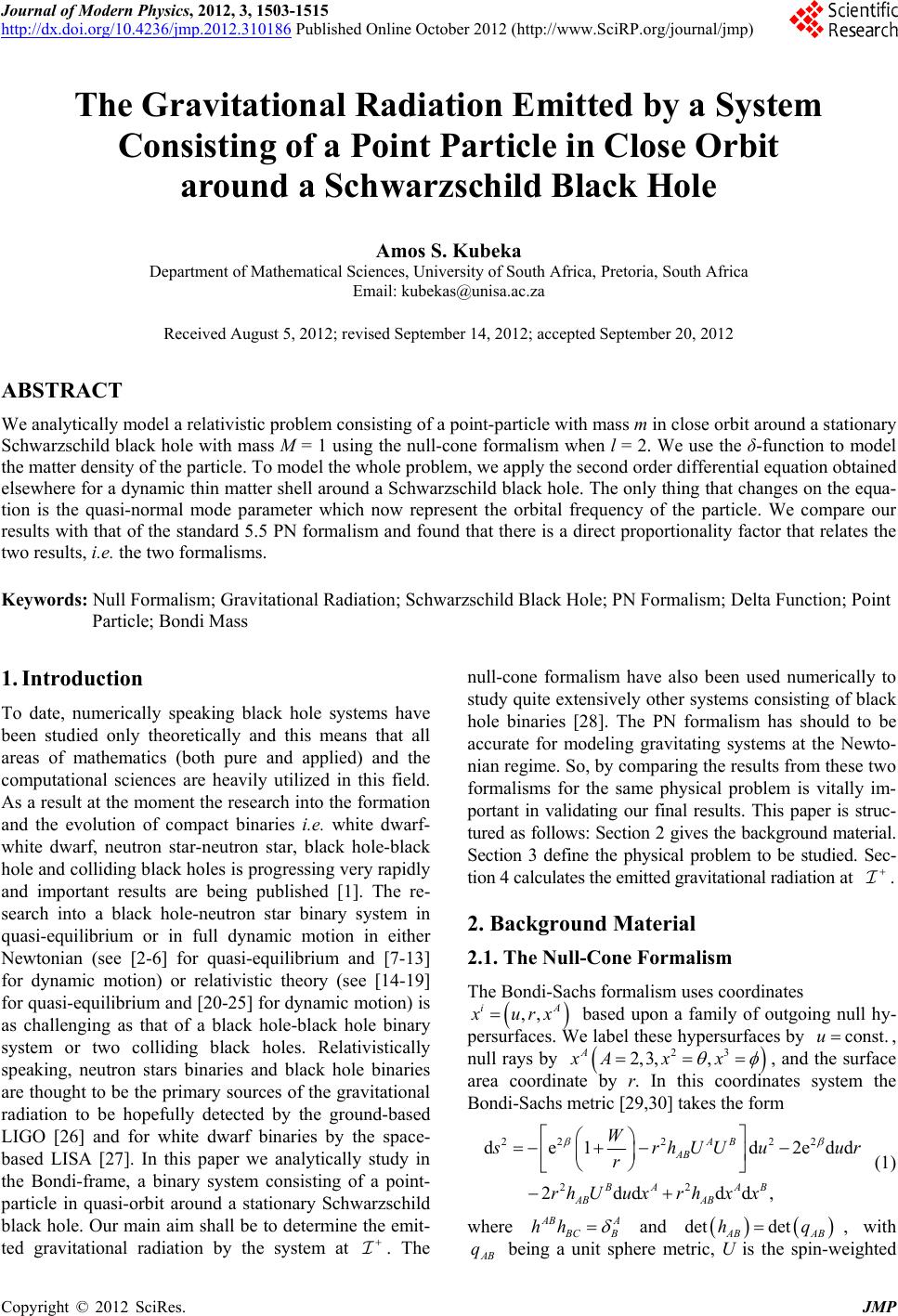
Journal of Modern Physics, 2012, 3, 1503-1515
http://dx.doi.org/10.4236/jmp.2012.310186 Published Online October 2012 (http://www.SciRP.org/journal/jmp)
The Gravitational Radiation Emitted by a System
Consisting of a Point Particle in Close Orbit
around a Schwarzschild Black Hole
Amos S. Kubeka
Department of Mathematical Sciences, University of South Africa, Pretoria, South Africa
Received August 5, 2012; revised September 14, 2012; accepted September 20, 2012
ABSTRACT
We analytically model a relativistic problem consisting of a point-particle with mass m in close orbit around a stationary
Schwarzschild black hole with mass M = 1 using the null-cone formalism when l = 2. We use the δ-function to model
the matter density of the particle. To model the whole problem, we apply the second order differential equation obtained
elsewhere for a dynamic thin matter shell around a Schwarzschild black hole. The only thing that changes on the equa-
tion is the quasi-normal mode parameter which now represent the orbital frequency of the particle. We compare our
results with that of the standard 5.5 PN formalism and found that there is a direct proportionality factor that relates the
two results, i.e. the two formalisms.
Keywords: Null Formalism; Gravitational Radiation; Schwarzschild Black Hole; PN Formalism; Delta Function; Point
Particle; Bondi Mass
1. Introduction
To date, numerically speaking black hole systems have
been studied only theoretically and this means that all
areas of mathematics (both pure and applied) and the
computational sciences are heavily utilized in this field.
As a result at the moment the research into the formation
and the evolution of compact binaries i.e. white dwarf-
white dwarf, neutron star-neutron star, black hole-black
hole and colliding black holes is progressing very rapidly
and important results are being published [1]. The re-
search into a black hole-neutron star binary system in
quasi-equilibrium or in full dynamic motion in either
Newtonian (see [2-6] for quasi-equilibrium and [7-13]
for dynamic motion) or relativistic theory (see [14-19]
for quasi-equilibrium and [20-25] for dynamic motion) is
as challenging as that of a black hole-black hole binary
system or two colliding black holes. Relativistically
speaking, neutron stars binaries and black hole binaries
are thought to be the primary sources of the gravitational
radiation to be hopefully detected by the ground-based
LIGO [26] and for white dwarf binaries by the space-
based LISA [27]. In this paper we analytically study in
the Bondi-frame, a binary system consisting of a point-
particle in quasi-orbit around a stationary Schwarzschild
black hole. Our main aim shall be to determine the emit-
ted gravitational radiation by the system at

. The
null-cone formalism have also been used numerically to
study quite extensively other systems consisting of black
hole binaries [28]. The PN formalism has should to be
accurate for modeling gravitating systems at the Newto-
nian regime. So, by comparing the results from these two
formalisms for the same physical problem is vitally im-
portant in validating our final results. This paper is struc-
tured as follows: Section 2 gives the background material.
Section 3 define the physical problem to be studied. Sec-
tion 4 calculates the emitted gravitational radiation at

.
2. Background Material
2.1. The Null-Cone Formalism
The Bondi-Sachs formalism uses coordinates


,,
iA
x
urx
const.u
based upon a family of outgoing null hy-
persurfaces. We label these hypersurfaces by

,
null rays by


23
2, 3,,
A
xAx x



, and the surface
area coordinate by r. In this coordinates system the
Bondi-Sachs metric [29,30] takes the form
22 222
22
de1 d2edd
2dd dd,
AB
AB
BA AB
AB AB
Wrh UUuur
r
rh Uuxrhx x




 



AB A
s
(1)
where
B
CB
hh


 
det dethq
AB
q
and ABAB , with
being a unit sphere metric, U is the spin-weighted
C
opyright © 2012 SciRes. JMP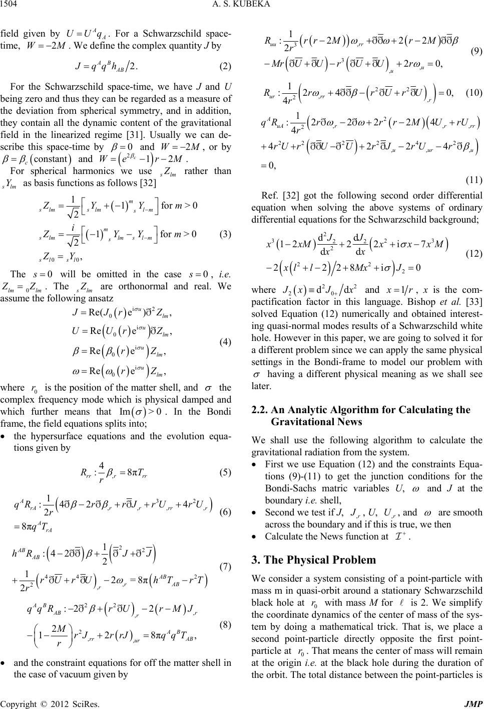

A. S. KUBEKA
1504
field given by A UU . For a Schwarzschild space-
time, . We define the complex quantity J by
Aq
M2W
  
2.
AB
AB
qqhJ (2)
For the Schwarzschild space-time, we have J and U
being zero and thus they can be regarded as a measure of
the deviation from spherical symmetry, and in addition,
they contain all the dynamic content of the gravitational
field in the linearized regime [31]. Usually we can de-
scribe this space-time by 0


an
2c
We


d , or by
and .
2WM

12rM

antcon st  c
For spherical harmonics we use
s
lm
Z
rather than
s
lm
Y as basis functions as follows [32]


00
1
2
1
2
,
m
1f or>0
for>0
m slmlm
s
m
mlm slm
s
sl
ZYYm
i
ZYYm
ZY






 


0 s
sl
sl
sl
0s
(3)
The will be omitted in the case

, i.e.
0lm lm
Z
Z. The
s
lm
Z
are orthonormal and real. We
assume the following ansatz







i2
i
i
i
e ),
e ,
e ,
e ,
u
lm
u
lm
u
lm
u
lm
0
0
0
0
Re(
Re
Re
Re
J
Jr
UU






Z
r Z
rZ
rZ






(4)
where 0 is the position of the matter shell, and r

the
complex frequency mode which is physical damped and
which further means that Im. In the Bondi
frame, the field equations splits into;

 > 0
 the hypersurface equations and the evolution equa-
tions given by
,
4
:8π
r rr
RT
r
 
rr (5)

32
, ,
:4 2 4
r r rrr
rrJ rUrU  
,,
1
2
8π
A
rA
A
rA
qR r
qT
(6)




22
44 2
,
,
1
22
2=8πAB
rA B
r
J J
rUrUhT rT



 
 



2
:4
1
2
AB
AB
hR
r
(7)

,
2
,,
2
12
AB r
rr ur
MrJ rrJ
r

 



22
,
:2 2
8π,
AB
r
AB
AB
qqRrUrMJ
qqT
  
 (8)
 and the constraint equations for off the matter shell in
the case of vacuum given by

,
3
3
,
,
1
:2 22
2
20,
uu rr
u
u
RrrM rM
r
MrU Ur U Ur






 
 
(9)



22
,
2,
1
:2 40,
4
ur rrr
Rr rUrU
r


  (10)

 
 
2
,,,
2
222 242
,, ,
1
:222 24
4
4224
0,
A
uArr rr
uuru
qRrr rMUrU
r
rU rUUrJrUr


 
 


 

(11)
Ref. [32] got the following second order differential
equation when solving the above systems of ordinary
differential equations for the Schwarzschild background;

 
2
323
22
2
22
2
dd
1222 i7
d d
2228i0
JJ
x
xMxxx M
x x
xl lMxJ




(12)


22
dd
J
where 20 xJx and
x
1r, x is the com-
pactification factor in this language. Bishop et al. [33]
solved Equation (12) numerically and obtained interest-
ing quasi-normal modes results of a Schwarzschild white
hole. However in this paper, we are going to solved it for
a different problem since we can apply the same physical
settings in the Bondi-frame to model our problem with

having a different physical meaning as we shall see
later.
2.2. An Analytic Algorithm for Calculating the
Gravitational News
We shall use the following algorithm to calculate the
gravitational radiation from the system.
 First we use Equation (12) and the constraints Equa-
tions (9)-(11) to get the junction conditions for the
Bondi-Sachs matric variables U,

and J at the
boundary i.e. shell,
 Second we test if J, ,r
J
, U, ,r U, and

are smooth
across the boundary and if this is true, we then
 Calculate the News function at  .
3. The Physical Problem
We consider a system consisting of a point-particle with
mass m in quasi-orbit around a stationary Schwarzschild
black hole at 0 with mass M for is 2. We simplify
the coordinate dynamics of the center of mass of the sys-
tem by doing a mathematical trick. That is, we place a
second point-particle directly opposite the first point-
particle at 0. That means the center of mass will remain
at the origin i.e. at the black hole during the duration of
the orbit. The total distance between the point-particles is
r
r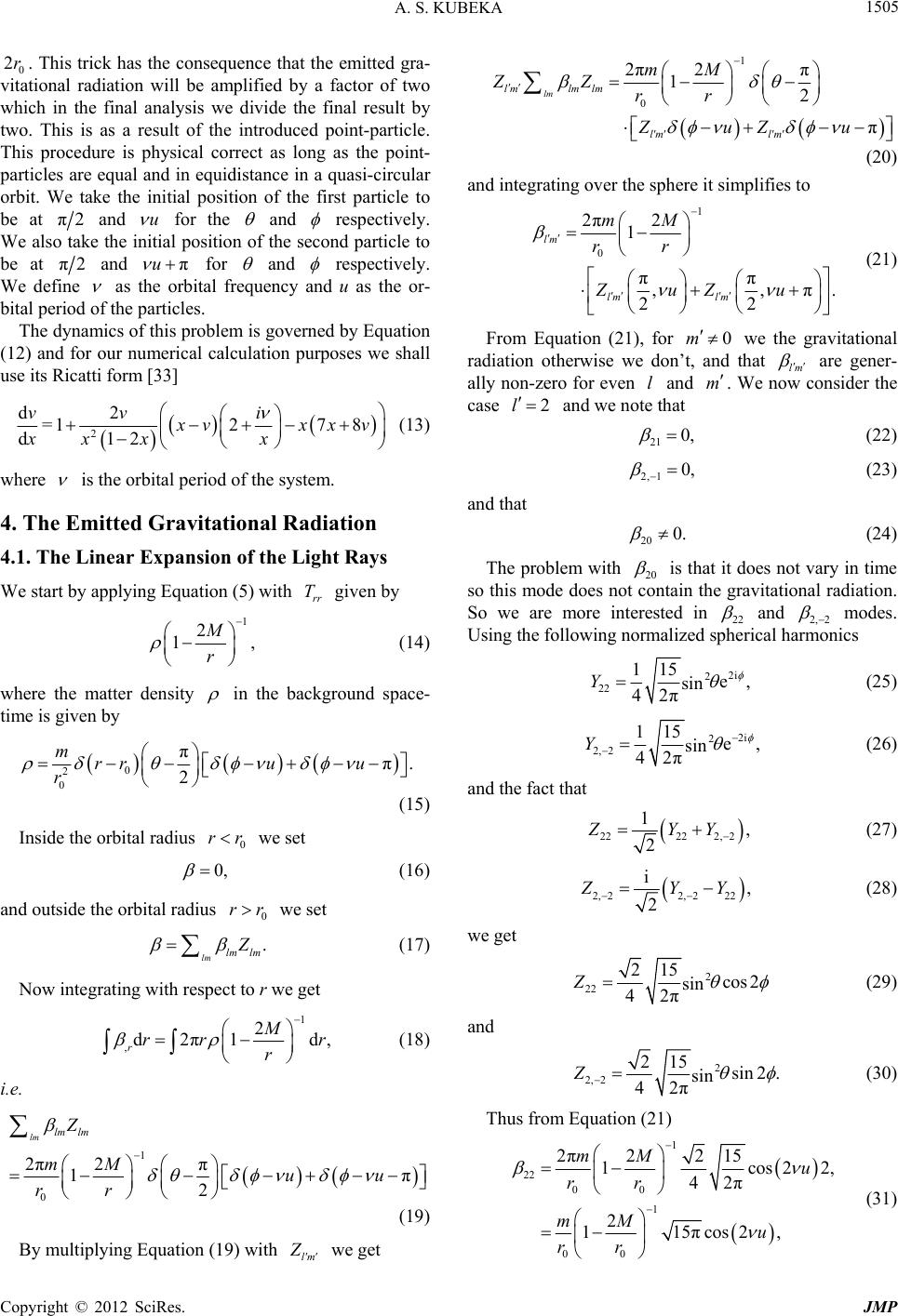

A. S. KUBEKA 1505
0. This trick has the consequence that the emitted gra-
vitational radiation will be amplified by a factor of two
which in the final analysis we divide the final result by
two. This is as a result of the introduced point-particle.
This procedure is physical correct as long as the point-
particles are equal and in equidistance in a quasi-circular
orbit. We take the initial position of the first particle to
be at
2r
π
 
1
0
2π2π
12
π
lm
l mlmlm
lm lm
mM
ZZ
rr
ZuZu

  


 

 



2 and u

for the

and

respectively.
We also take the initial position of the second particle to
be at π2 and πu

 for

and

respectively.
We define

as the orbital frequency and u as the or-
bital period of the particles.
The dynamics of this problem is governed by Equation
(12) and for our numerical calculation purposes we shall
use its Ricatti form [33]

 
2
d2 278
d12
vv i
=1
x
vxxv
xx
 


 


xx
 (13)
where

is the orbital period of the system.
4. The Emitted Gravitational Radiation
4.1. The Linear Expansion of the Light Rays
We start by applying Equation (5) with given by
rr
T
1
,




2
1
M
r


 (14)
where the matter density

in the background space-
time is given by
  
0
2
ππ.
2
rru u
 

 




0
r
0
m
r
r
(15)
Inside the orbital radius

we set
0,


lm
(16)
and outside the orbital radius we set
0
rr
lmlm .
Z
  (17)
Now integrating with respect to r we get
1
2
1d,
Mr
r





,d2π

rrr
 (18)
i.e.

2
1π
lm
Z
mM uu
rr
  

 
1
0
2π
lm lm

π
2








lm
(19)
By multiplying Equation (19) with
Z

we get





(20)
and integrating over the sphere it simplifies to
1
0
2π2
1
ππ
,,π.
22
lm
lm lm
mM
rr
ZuZu




 






 

 
(21)


 


0m
From Equation (21), for we the gravitational
radiation otherwise we don’t, and that lm


are gener-
ally non-zero for even and m. We now consider the
case
l
2l


and we note that
(22)
21 0,


(23)
2, 10,



and that
(24)
20 0.


The problem with 20

is that it does not vary in time
so this mode does not contain the gravitational radiation.
So we are more interested in 22

and 2, 2


modes.
Using the following normalized spherical harmonics
2i
2
22
115 e,
sin
42π
Y

(25)  
2i
2
2, 2
115 e,
sin
42π
Y 



(26)
and the fact that

22222, 2
1,
2
ZYY

 (27)

2, 22, 222
i,
2
ZYY

 (28)
we get
2
22
215 cos 2
sin
42π
Z

  (29)
and
2
2, 2
215 sin 2
sin
42π
Z.


 (30)
Thus from Equation (21)


1
22
00
1
00
2π2215
1cos22,
42π
2
115πcos 2,
mM u
rr
mM u
rr












(31)

A. S. KUBEKA
1506
and similarly

5πsin2 u
1
2, 2
00
2
11
mM
rr







 (32)
and then finally we write

1
00
2i
22
2
15π1
Re eRe
mM
rr







 

2i
2, 2
ie
uu
ZZ



1
(33)
Now taking
M
, Equation (35) then becomes


1
00
2i
22
2
15π1
Re eRe
m
rr







 

2i
2, 2
ie
uu
ZZ



(34)
Finally, we divide Equation (34) by a factor of 2 to
appropriate it for a single point-particle in orbit around a
Schwarzschild black hole. We are able to do this because
for π20

0Z we have 2,1. Therefore from here
onwards, the calculations will be that of a single point-
particle. Equation (34) now becomes

1
00
2i
22
12
15π1
2
Re eRe
m
rr







  
2i
2, 2
ie
uu
ZZ



6rr

(35)
4.2. The Gravitational Radiation
We assume that the orbit is at the innermost stable circu-
lar orbit (ISCO), so that 0. We then found the
change in the Schwarzschild coordinate time for one
complete revolution of 92.3436 from which we found the
orbital frequency

of 0.0680.
To now find the numerical solutions to continue Equa-
tion (13) we make the spatial coordinate transformation
of 1
x
r which then imply that the ISCO is now at
16x
 
<< 0.5,
mn
xx


mn . The numerical computations are done in the
domains

0 <<and
mn
DxxD

 (36)
with numerical solutions


vx
 and  respec-
tively. We start the calculation with the transformed Eq-
uation (12) given by

vx
 



 
i
Jx
Jx
3
4
03
2
32
2
2
1d
212
2d
d
2i
d
d
22 i
d
UxxxxM x
xx xMx
x
xxMJxJx
x


 
 
   

x

Ux

(37)
where , are the Bondi metric functions,
and 0
U



, 0


are the values of the expansion of the
light rays

given by Equation (35) in the exterior and
interior domains respectively. N.B the derivatives of J
should not be worked out numerically, but should be
worked out analytically in terms of 1
J
, 2
J
and
from Equation (13) to be found with
v
0.0680

.

We define the general solutions for 2
J
xmn at
x
outside and inside the orbital radius respectively as


0
41 2,
J
xccxcJx

  (38)


0
96 7,
J
xccxcJx


4c1c29 , 6
(39)
where , , c, ccand 7care constants to
be determined numerically. The functions


0
J
x
 and


0
J
x aren analytic near m
x
a
  
nd therefore can be
Taylor expand as





00
23
23
00
d
d
dd
,
2d 6d
mn mn
mn mn
JxJ xxxJx
x
xxxx
J
xJx
x
x
 




  
(40)





00
23
23
00
d
d
dd
,
2d 6d
mn mn
mn mn
JxJ xxxJ x
x
xx xx
J
xJx
x
x
 




(41)
which then results in Equations (38) and (41) being ana-
lytic near mn
x
. We used Matlab ode45 solver to find
numerical solutions of the above derivatives in Equations
(40) and (41). We used stringent numerical conditions to
get the results to about seven significant figures with
RelTol of 12
10

, AbsTol of , and the MaxStep of
12
10
6
210

 and the results we found to be

5
0
d291442.28067210 i,
dJx
  (42)
x

2
67
0
d2.865551101.5233513010 i,
dJx
 (43)
x

3
79
0
d4.8870101.859143110 i,
dJx
 
(44)
x
and

0
d13.04337 1.31529i,
dJx
 (45)
x

2
21
0
d1.54689103.1998010i,
dJx

(46)
x

3
33
0
d1.12428101.2531110 i
dJx .
  (47)
x
We have tested for the consistency of the above results
by using other Matlab solvers; ode23 and ode15s (which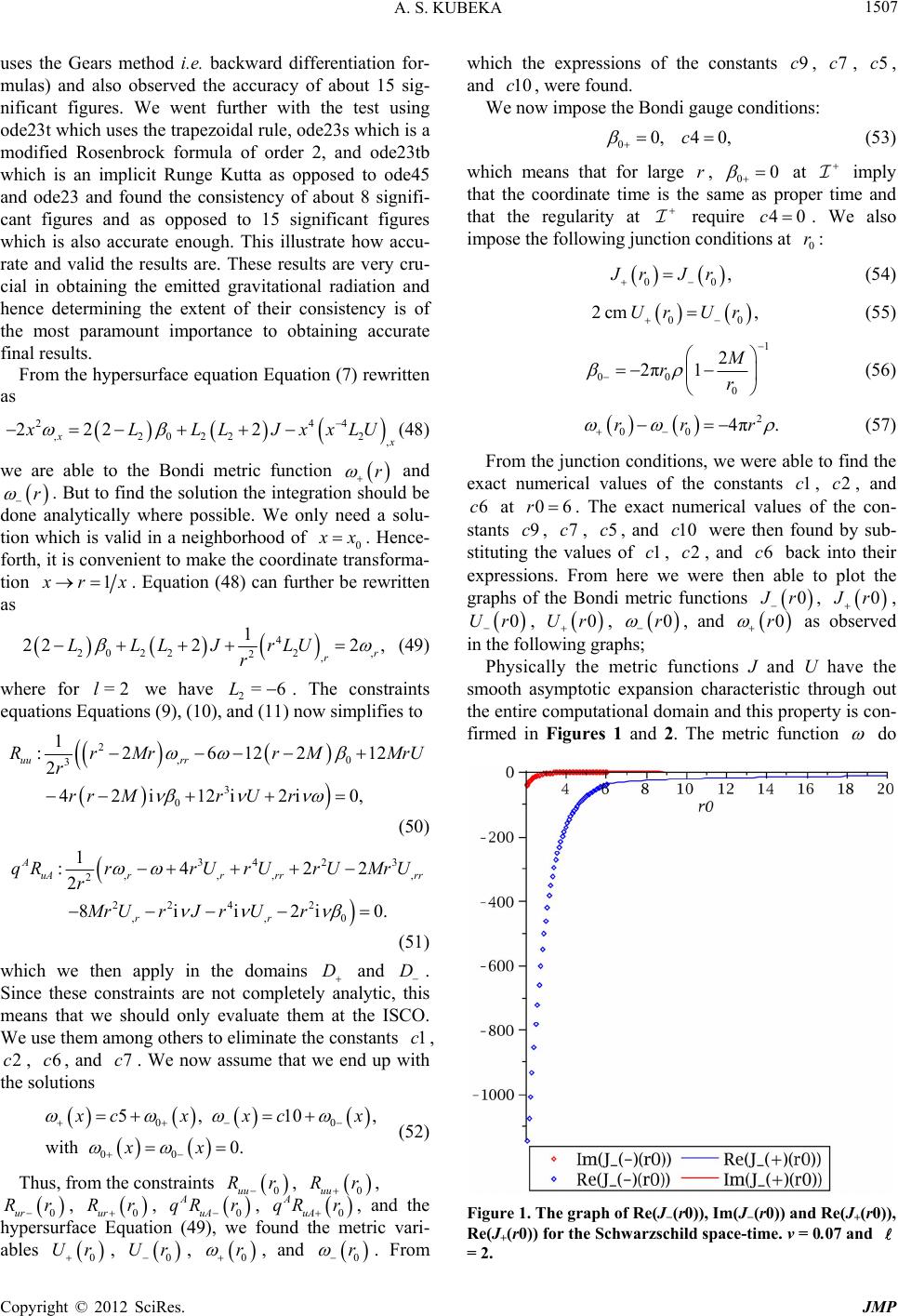

A. S. KUBEKA 1507
uses the Gears method i.e. backward differentiation for-
mulas) and also observed the accuracy of about 15 sig-
nificant figures. We went further with the test using
ode23t which uses the trapezoidal rule, ode23s which is a
modified Rosenbrock formula of order 2, and ode23tb
which is an implicit Runge Kutta as opposed to ode45
and ode23 and found the consistency of about 8 signifi-
cant figures and as opposed to 15 significant figures
which is also accurate enough. This illustrate how accu-
rate and valid the results are. These results are very cru-
cial in obtaining the emitted gravitational radiation and
hence determining the extent of their consistency is of
the most paramount importance to obtaining accurate
final results.
From the hypersurface equation Equation (7) rewritten
as
 
,2
022
222 2
x

244
2
,
x
x
LLL  JxxLU

(48)
we are able to the Bondi metric function


r 

r 
 and
. But to find the solution the integration should be
done analytically where possible. We only need a solu-
tion which is valid in a neighborhood of 0
x
x. Hence-
forth, it is convenient to make the coordinate transforma-
tion 1
x
rx . Equation (48) can further be rewritten
as
 

2 ,
,2,
r
r
rLU
4
20 222
1
22 2LLLJ
r

 
=6L
 (49)
where for l we have 2. The constraints
equations Equations (9), (10), and (11) now simplifies to
=2





2
3
3
0
1
:2612
2
42i12i2i
uu rr
RrMrr M
r
rrMr Ur

 

 
,0
212
0,
MrU  

(50)

34
,,,
2
22 4
,,
1
:4
2
8ii
A
uArr rr
rr
qRrrU rUr
r
Mr UrJrUr


 


2 3
,
2
0
22
2i0.
rr
U MrU



D D
(51)
which we then apply in the domains  and

.
Since these constraints are not completely analytic, this
means that we should only evaluate them at the ISCO.
We use them among others to eliminate the constants ,
, , and . We now assume that we end up with
the solutions
1c
6c7c2c
 


00
10,
 
00
5,
with 0.
x
cxx
xx




 

c x 



0
r

uu
Rr

(52)
Thus, from the constraints , 0,
0ur, ur ,

uu
R


R

rR

0
r


0
r

A
qR

0
Ur

uA , 0 uA, and the
hypersurface Equation (49), we found the metric vari-
ables , ,

A
qR r

0
Ur



0
r 
, and . From
which the expressions of the constants c, , ,
and , were found.

0
r 

9 7c5c
10c
00,4 0,c
We now impose the Bondi gauge conditions:




r0
(53)

which means that for large , 0

 at  imply
that the coordinate time is the same as proper time and
that the regularity at

40c
0
r
require . We also
impose the following junction conditions at :


00
,
J
rJr

 (54)


00
2cm ,Ur Ur

 (55)
1
00
0
2
2π1M rr 



 


(56)




2
00
4πrrr

. 


1c2c
6c06r
(57)
From the junction conditions, we were able to find the
exact numerical values of the constants , , and
at

. The exact numerical values of the con-
stants , , , and were then found by sub-
stituting the values of , , and back into their
expressions. From here we were then able to plot the
graphs of the Bondi metric functions
9c7c5c10c
1c2c6c




0
J
0r
,
J
r
,


0Ur
,


0Ur
,


0r 

0r 
 , and as observed
in the following graphs;
Physically the metric functions J and U have the
smooth asymptotic expansion characteristic through out
the entire computational domain and this property is con-
firmed in Figures 1 and 2. The metric function

do
Figure 1. The graph of Re(J−(r0)), Im(J−(r0)) and Re(J+(r0)),
Re(J+(r0)) for the Schwarzschild space-time. ν = 0.07 and
= 2.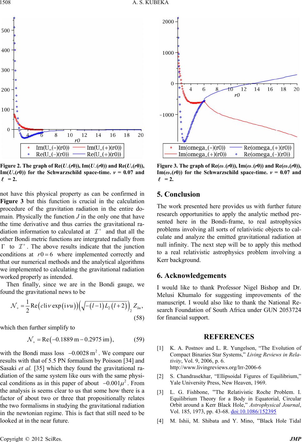


A. S. KUBEKA
1508
Figure 2. The graph of Re(U−(r0)), Im(U−(r0)) and Re(U+(r0)),
Im(U+(r0)) for the Schwarzschild space-time. ν = 0.07 and
= 2. 


Γ 
06r
not have this physical property as can be confirmed in
Figure 3 but this function is crucial in the calculation
procedure of the gravitation radiation in the entire do-
main. Physically the function J in the only one that have
the time derivative and thus carries the gravitational ra-
diation information to calculated at and that all the
other Bondi metric functions are intergrated radially from
to . The above results indicate that the junction
conditions at where implemented correctly and
that our numerical methods and the analytical algorithms
we implemented to calculating the gravitational radiation
worked properly as intended.
Then finally, since we are in the Bondi gauge, we
found the gravitational news to be


 


2
2 ,
lm
LlZ

0.2975 im,
2
1Re1iexp i1
2cul


(58)
which then further simplify to
Re0.1889 m


(59)
with the Bondi mass loss . We compare our
results with that of 5.5 PN formalism by Poisson [34] and
Sasaki et al. [35] which they found the gravitational ra-
diation of the same system like ours with the same physi-
cal conditions as in this paper of about
Figure 3. The graph of Re(ω−(r0)), Im(ω−(r0)) and Re(ω+(r0)),
Im(ω+(r0)) for the Schwarzschild space-time. ν = 0.07 and
= 2. 
5. Conclusion
The work presented here provides us with further future
research opportunities to apply the analytic method pre-
sented here in the Bondi-frame, to real astrophysics
problems involving all sorts of relativistic objects to cal-
culate and analyze the emitted gravitational radiation at
null infinity. The next step will be to apply this method
to a real relativistic astrophysics problem involving a
Kerr background.
6. Acknowledgements
I would like to thank Professor Nigel Bishop and Dr.
Melusi Khumalo for suggesting improvements of the
manuscript. I would also like to thank the National Re-
search Foundation of South Africa under GUN 2053724
for financial support.
REFERENCES
[1] K. A. Postnov and L. R. Yungelson, “The Evolution of
Compact Binaries Star Systems,” Living Reviews in Rela-
tivity, Vol. 9, 2006, p. 6.
http://www.livingreviews.org/lrr-2006-6
2
0.0028m
2
0.001
[2] S. Chandrasekhar, “Ellipsoidal Figures of Equilibrium,”
Yale University Press, New Heaven, 1969.

. From
the analysis is seems clear to us that some how there is a
factor of about two or three that propositionally relates
the two formalisms in studying the gravitational radiation
in the newtonian regime. This is fact that still need to be
looked at in the near future.
[3] L. G. Fishbone, “The Relativistic Roche Problem. I.
Equilibrium Theory for a Body in Equatorial, Circular
Orbit around a Kerr Black Hole,” Astrophysical Journal,
Vol. 185, 1973, pp. 43-68. doi:10.1086/152395
[4] M. Ishii, M. Shibata and Y. Mino, “Black Hole Tidal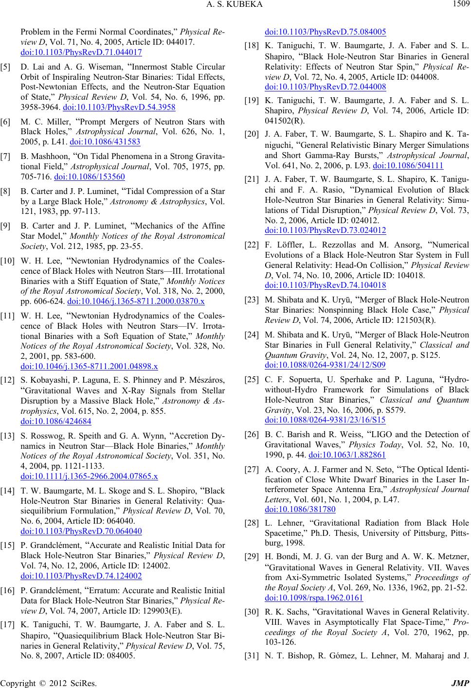

A. S. KUBEKA 1509
Problem in the Fermi Normal Coordinates,” Physical Re-
view D, Vol. 71, No. 4, 2005, Article ID: 044017.
doi:10.1103/PhysRevD.71.044017
[5] D. Lai and A. G. Wiseman, “Innermost Stable Circular
Orbit of Inspiraling Neutron-Star Binaries: Tidal Effects,
Post-Newtonian Effects, and the Neutron-Star Equation
of State,” Physical Review D, Vol. 54, No. 6, 1996, pp.
3958-3964. doi:10.1103/PhysRevD.54.3958
[6] M. C. Miller, “Prompt Mergers of Neutron Stars with
Black Holes,” Astrophysical Journal, Vol. 626, No. 1,
2005, p. L41. doi:10.1086/431583
[7] B. Mashhoon, “On Tidal Phenomena in a Strong Gravita-
tional Field,” Astrophysical Journal, Vol. 705, 1975, pp.
705-716. doi:10.1086/153560
[8] B. Carter and J. P. Luminet, “Tidal Compression of a Star
by a Large Black Hole,” Astronomy & Astrophysics, Vol.
121, 1983, pp. 97-113.
[9] B. Carter and J. P. Luminet, “Mechanics of the Affine
Star Model,” Monthly Notices of the Royal Astronomical
Society, Vol. 212, 1985, pp. 23-55.
[10] W. H. Lee, “Newtonian Hydrodynamics of the Coales-
cence of Black Holes with Neutron Stars—III. Irrotational
Binaries with a Stiff Equation of State,” Monthly Notices
of the Royal Astronomical Society, Vol. 318, No. 2, 2000,
pp. 606-624. doi:10.1046/j.1365-8711.2000.03870.x
[11] W. H. Lee, “Newtonian Hydrodynamics of the Coales-
cence of Black Holes with Neutron Stars—IV. Irrota-
tional Binaries with a Soft Equation of State,” Monthly
Notices of the Royal Astronomical Society, Vol. 328, No.
2, 2001, pp. 583-600.
doi:10.1046/j.1365-8711.2001.04898.x
[12] S. Kobayashi, P. Laguna, E. S. Phinney and P. Mészáros,
“Gravitational Waves and X-Ray Signals from Stellar
Disruption by a Massive Black Hole,” Astronomy & As-
trophysics, Vol. 615, No. 2, 2004, p. 855.
doi:10.1086/424684
[13] S. Rosswog, R. Speith and G. A. Wynn, “Accretion Dy-
namics in Neutron Star—Black Hole Binaries,” Monthly
Notices of the Royal Astronomical Society, Vol. 351, No.
4, 2004, pp. 1121-1133.
doi:10.1111/j.1365-2966.2004.07865.x
[14] T. W. Baumgarte, M. L. Skoge and S. L. Shopiro, “Black
Hole-Neutron Star Binaries in General Relativity: Qua-
siequilibrium Formulation,” Physical Review D, Vol. 70,
No. 6, 2004, Article ID: 064040.
doi:10.1103/PhysRevD.70.064040
[15] P. Grandclément, “Accurate and Realistic Initial Data for
Black Hole-Neutron Star Binaries,” Physical Review D,
Vol. 74, No. 12, 2006, Article ID: 124002.
doi:10.1103/PhysRevD.74.124002
[16] P. Grandclément, “Erratum: Accurate and Realistic Initial
Data for Black Hole-Neutron Star Binaries,” Physical Re-
view D, Vol. 74, 2007, Article ID: 129903(E).
[17] K. Taniguchi, T. W. Baumgarte, J. A. Faber and S. L.
Shapiro, “Quasiequilibrium Black Hole-Neutron Star Bi-
naries in General Relativity,” Physical Review D, Vol. 75,
No. 8, 2007, Article ID: 084005.
doi:10.1103/PhysRevD.75.084005
[18] K. Taniguchi, T. W. Baumgarte, J. A. Faber and S. L.
Shapiro, “Black Hole-Neutron Star Binaries in General
Relativity: Effects of Neutron Star Spin,” Physical Re-
view D, Vol. 72, No. 4, 2005, Article ID: 044008.
doi:10.1103/PhysRevD.72.044008
[19] K. Taniguchi, T. W. Baumgarte, J. A. Faber and S. L.
Shapiro, Physical Review D, Vol. 74, 2006, Article ID:
041502(R).
[20] J. A. Faber, T. W. Baumgarte, S. L. Shapiro and K. Ta-
niguchi, “General Relativistic Binary Merger Simulations
and Short Gamma-Ray Bursts,” Astrophysical Journal,
Vol. 641, No. 2, 2006, p. L93. doi:10.1086/504111
[21] J. A. Faber, T. W. Baumgarte, S. L. Shapiro, K. Tanigu-
chi and F. A. Rasio, “Dynamical Evolution of Black
Hole-Neutron Star Binaries in General Relativity: Simu-
lations of Tidal Disruption,” Physical Review D, Vol. 73,
No. 2, 2006, Article ID: 024012.
doi:10.1103/PhysRevD.73.024012
[22] F. Löffler, L. Rezzollas and M. Ansorg, “Numerical
Evolutions of a Black Hole-Neutron Star System in Full
General Relativity: Head-On Collision,” Physical Review
D, Vol. 74, No. 10, 2006, Article ID: 104018.
doi:10.1103/PhysRevD.74.104018
[23] M. Shibata and K. Uryū, “Merger of Black Hole-Neutron
Star Binaries: Nonspinning Black Hole Case,” Physical
Review D, Vol. 74, 2006, Article ID: 121503(R).
[24] M. Shibata and K. Uryū, “Merger of Black Hole-Neutron
Star Binaries in Full General Relativity,” Classical and
Quantum Gravity, Vol. 24, No. 12, 2007, p. S125.
doi:10.1088/0264-9381/24/12/S09
[25] C. F. Sopuerta, U. Sperhake and P. Laguna, “Hydro-
without-Hydro Framework for Simulations of Black
Hole-Neutron Star Binaries,” Classical and Quantum
Gravity, Vol. 23, No. 16, 2006, p. S579.
doi:10.1088/0264-9381/23/16/S15
[26] B. C. Barish and R. Weiss, “LIGO and the Detection of
Gravitational Waves,” Physics Today, Vol. 52, No. 10,
1990, p. 44. doi:10.1063/1.882861
[27] A. Coory, A. J. Farmer and N. Seto, “The Optical Identi-
fication of Close White Dwarf Binaries in the Laser In-
terferometer Space Antenna Era,” Astrophysical Journal
Letters, Vol. 601, No. 1, 2004, p. L47.
doi:10.1086/381780
[28] L. Lehner, “Gravitational Radiation from Black Hole
Spacetime,” Ph.D. Thesis, University of Pittsburg, Pitts-
burg, 1998.
[29] H. Bondi, M. J. G. van der Burg and A. W. K. Metzner,
“Gravitational Waves in General Relativity. VII. Waves
from Axi-Symmetric Isolated Systems,” Proceedings of
the Royal Society A, Vol. 269, No. 1336, 1962, pp. 21-52.
doi:10.1098/rspa.1962.0161
[30] R. K. Sachs, “Gravitational Waves in General Relativity.
VIII. Waves in Asymptotically Flat Space-Time,” Pro-
ceedings of the Royal Society A, Vol. 270, 1962, pp.
103-126.
[31] N. T. Bishop, R. Gómez, L. Lehner, M. Maharaj and J.

A. S. KUBEKA
1510
Winicour, “High-Powered Gravitational News,” Physical
Review D, Vol. 56, No. 10, 1997, pp. 6298-6309.
doi:10.1103/PhysRevD.56.6298
[32] N. T. Bishop, “Linearized Solutions of the Einstein Equa-
tions within a Bondi-Sachs Framework, and Implications
for Boundary Conditions in Numerical Simulations,”
Classical and Quantum Gravity, Vol. 22, No. 12, 2005, p.
2393. doi:10.1088/0264-9381/22/12/006
[33] N. T. Bishop and A. S. Kubeka, “Quasinormal Modes of
a Schwarzschild White Hole,” Physical Review D, Vol.
80, No. 6, 2009, Article ID: 064011.
doi:10.1103/PhysRevD.80.064011
[34] E. Poisson, “Gravitational Radiation from a Particle in
Circular Orbit around a Black Hole. I. Analytical Results
for the Nonrotating Case,” Physical Review D, Vol. 47,
No. 4, 1993, p. 1497. doi:10.1103/PhysRevD.47.1497
[35] M. Sasaki and H. Tagoshi, “Analytic Black Hole Pertur-
bation approach to Gravitational Radiation,” Living Re-
views in Relativity, Vol. 6, 2003, p. 6.

A. S. KUBEKA 1511
The Constraints Computed at
0
r
7
5
10
7 0
c
cr
19 2
5
10i 7 0
7 0
ccr
cr
8 6
10 i010
r
r c
5
6
0 6
0
c
r
cr
 

157
0 ln07
7 0
rrc
r



991937
0
1649 617
11 5894
1.00000000010200 076.00535857510i 7 06.800000010i 0
1.292409115 10iln0703.000000000 101006.692070654 10
1.440000000 10091000i704.896000000 10i0
uu
Rrrccr r
rcrcr
rc crr


 


16 79 617
194811 8
10 787
6 3.227234492
2.084590843 10704.896000000 10i907.215316909 10 ln0
1.04471038510i 071000 071.884955592100
3.600000000 10098.16000000 10i063.41805
cr crr
rc rcr
rc rc






97
98 96117
17 419 39
17 617
280810 i 0
6.83610561310 i 04.48800000010i063.015928948100
7.179615196107 01.098242223107 020000i072.72000000
1.80602632310ln07 02.16389824710i
r
rrc
crcrr c
rcrc





 


69
17416611
1910518 5
16 6
708.16000000010i
7.212387448 10 ln0708.346481884 10701.507964474 10
2.1111840001071.2000000001010 01.38291806710i7 0
1.31170554210i0 ln074.896000000
rr
rcrcr
ccr
rrc

 

 

95
1913 720
11 616799
19 2
10 i 904.08701955310i
1.741939934107 07.323651653100ln076.49175424910i
1.440000000 10094.113828618 10i702.563539606 10i0
1.65027134910703.4239
cr
crrrcc
rccrrp
cr

 






15 520
2
10 47
8706 10i0ln078.031498194 10i
1.2000000001010 0002,
rrc
crr r

 
7c
(60)



23
0
45 4
233
12020915.9586340i 200.8160000000i 40.6052309472 2
6745.674492 2080948.09432 207518.667272i 2090224.00728i 2
1.503112547i 269.78185262i 202733.489212 20121036.078
uu
Rrr rcrcc
crcr cr cr
ccrcrcr
 
 

5
0


2
2
2 20
793170i 20
cr
cr
2 2
32
3
1900
7518.667272i 2053.40273063i 200.1360i 01253.111212i 20457.9
7518.667272i 200.3026154736 2 022.10459629 2 01124.279082 20
6745.674528 2012 0 48.900455105i 2 0
crcr rcr
crcrcrc r
cr rccr






2
3
62734i 2 0
72 0 4
cr
rc


2
22
69.78185262iln02 0.75155
0.4080000000i041366.7446062061036.07819002ln025
1.815692842 2 0132.6275777 2 06745.674492 2040474.04717 20
2747.875902i 2045112.003
rc
rccrcrrc c
crcrc rc r
cr


 




32
11
0r
11 1
21
63i 20418.6911157iln024.509337640i 2
8200.4676362036 10216.4691401ln0265
1200.5043591226 1022.568292000 10209.800840000 10i20
50.692890582 00.68010i4 201.04797
crrc c
crcrr cc
r ccrcr
cr c



 




3
53 4
523 4
31 11
21i 200.1252593789i 2
6745.6745282 0228.55427452 01687.678839i2 038.40352765i2
7518.667272i2 02102102614.5469742 0
0.8160i00.5043591226 1022.568292000 10209.80
cr c
cr crcrcr
c rcrcrc r
rccr


 


2
0
11
21 3
53 4
523
0840000 10i
50.692890582 00.68010i4 201.0479721i2 00.1252593789i2
6745.6745282 0228.55427452 01687.678839i2 038.40352765i2
7518.667272i202 102 102614.5469742
cr ccrc
cr crcrcr
c rcrcrc r



 
 

2
2 0
0
cr

42
02.448000000i04rc3 0 ,r
(61)

A. S. KUBEKA
1512


919220
0
18 3620
518172
1.111111111101.27277425610i 7 01.31498977210i 70
1.58999851310i 7 076i 703.01181182210i74.846534181
40952i 077.9169400031072.28072197510703.6
ur
R rcrcr
cr crc
rc ccr







14 4
10i 7 0cr
18
051070cr
16 35 55 6
10 61646
163617
8.260193057107 03.02160107 01.510801070
3.3929200661002.70464529110 70002,
crcr cr
rcrrr 
 
 
(62)

 
3
0
545
233
120915.9586340i 200.8160000000i 40.6052309472 26745.674
80948.09432 207518.667272i 2090224.00728i 201.5031125
69.78185262i 202733.48921220121036.07819002
ur
Rr rcrcc
cr cr cr
crcrcr
 
 

4
492 20
47i 2
cr
c


2
2112112
464
3634
20
6 02.56829200010209.80084000010i 20101.3857812
603.1439163i2 033728.372642 0685.66282352 06750.7153
76.80705530i2037593.33636i204106 1010458.
cr
rcr cr
cr cr cr
crcrcr cr




3
5
2 0
56i 20
cr
cr 


5
11
2 0
i 20
2
cr
cr
c


11 1
21 3
534
18790
1200.5043591226 1022.568292000 10209.800840000 10
50.692890582 00.68010i4 201.0479721i2 00.1252593789i
6745.674528 20228.5542745 201687.678839i 2038.
rc cr
cr ccr
cr crcr



 
 


2
765i 20cr
1086 8184
4
7 0
A
cr

21 2
i 7 0cr

94
5
i 06
7 0
rc
cr


523 42
40352
7518.667272i202 102 102614.546974200,cr crcrcr r
(63)



0
20 15 718
19 520 3
1.0000000001016000i 7 01.00000010076.95123928107 0
4.6081851610i 7 06.81169926110i 7 01.20206457410ln0
1.14019952910i 7 07.39176465110i 7 01.22060
uA
qRrcrrccr
crcrr
cr cr
 
  




14 7
21 7156
10 4165
9 6176
8500107 0
4.461943440 10 i730005.385037980 10iln070
2.000000000 101002.154015192 10 iln0702.671516126 10
2.040000000 10i063.005161436 10 ln0708.1600000
cr
crp rcr
crr cr
rc rcr


 
 

10 59618
18516 6193
20 2164
00 10
2.000000000 101005.000000000 101001.202064574 10ln0
3.817318694107 06.54302141210i 078.8094050891070
1.455381063107 02.15401519210iln07 0
cr crr
crrccr
crr cr





19
959917 6
20 4209 8
1.44797289 10
8.16000000010i064.27256600910i 03.5095510261070
1.00141852810i 071.1728800001078.54513201810i 0
rc rcr
rcc r




 2
6
7 0
00 2,
cr
r r

(64)



222
2112
121253.111212i 2051124.279082 200.3026154736 2 0
2 0
A
qRrc rccrcr
c r

 

0
11 2 34
22.10459629 2 012 0436.07819002ln02802.56829200010
9.80084000010i 20101.3857812 20603.1439163i 20
33728
uA
cr rcr cr
cr crcr



 
 



6453
634 5
2
.372642 0685.66282352 06750.715356i2 076.807055
37593.33636i2 041061010458.187902 0
0 457.9793170i 200.8160000000i0 48.900455105i 20.605230
22.10459629 222
cr crcr
c rcrcrc r
rcrrc c
c
 



30i 20
9472 2 0
cr
cr

34
4
22
48.558164 2020237.02358 201242506.222
22556.00182i 201.503112547i 2 069.78185262i 20
1366.744606 2061036.07819002 20
crcr c
crcr cr
cr crcr



3
424i 20cr

A. S. KUBEKA 1513

3112 112
464
3634
402.568292000 10209.800840000 1020101.38578122
603.1439163i2 033728.372642 0685.66282352 06750.715356i
76.80705530i2037593.33636i204106 1010458.18790
rcr cr
cr cr cr
crcrcr crc




3
5
0
2 0
cr
cr


5
4
6
20
0
7678 20
r
cr
icr

41 13103
557 5
4574
05.136584000102 01.96016800010i2 0304.15734362
2412.575665i2 02.02370235810 2 02742.6512942 033753.5
230.4211659i202.25560018210 i2012 10241
rcrcr
crcr cr
crcrcrcr

 




56
950 20
0
cr
cr


21 1111
21 3
53
0 52290.93
200.5043591226 1022.568292000 10209.800840000 10i2
50.69289058 200.68010i 4201.0479721i 200.1252593789i 2
6745.674528 20228.5542745 201687.678839
rc cr
cr ccrc
crcr i







 


523 4
2
2
2 038.40352765i
7518.667272i202 102 102614.546974208.900455105i
0.2720i041 02113.04336905144130 1.31528646137769i10
77.34402850 15.99899824i10 16187.37984802
cr
cr crcrcr
rccrc r
r

 
 
 

42
2 0
2 0
1 6
cr
cr





3
01 6
2 0
r
cr

14 11 2
11 234
64 5
08.8518687i 1
457.9793170i200.680 10i02.568292000 1020
9.80084000010i2 0101.38578122 0603.14391632 0
33728.37264 20685.6628235 206750.715356i 2076.80705530i
cr rcr
cr cr icr
cr crcr


  
 
 



3
4
0cr
634 5
32
3113103
5
37593.33636i204 106 1010458.1879020
7518.667272i 2069.78185262iln020.7515562734i 20
2 05.13658400010201.96016800010i 20304.1573436 2
2412.575665i 202.0237
cr cr crcr
crrc cr
rcrcr
cr



 


57 5
45745
23
0235810 2 02742.6512942 033753.5
230.4211659i202.25560018210 i2012 10241052290.93
0.4080000000i046745.674528201366.74460620 6100,
cr cr
crcr crcr
rccrcrcr r




6
6
2
7678i 20
950 20
cr
cr
(65)
The Bondi Metric Variables Computed at r0

111 11
4
0
9i 2
52765i
r
c
c
 

0
21 3
53
0.5043591226 1022.568292000 10209.800840000 10i2
50.692890582 00.68010i4 201.0479721i2 00.125259378
6745.6745282 0228.55427452 01687.678839i2 038.403
Urccrc
cr ccr
cr crcr



 
 2
20r


523 4
7518.667272i202 102102614.54697420,c rcrcrcr
(66)






 
0
67
79
78
5
472.865551000 101.523351300 10i
4.887000002 101.859143100 10i1 0
2.443500001109.29571550010i70
267291442.28067200010i
2.865551000
c
cr
cc

 

 
 


795
4
4
4.887000002 101.859143100 10i70
1 60
Ur cr
rr






 

67
78
101.52335130010 i10
2.443500001109.29571550210 i10
r 
 23
1 6
1 60rr



A. S. KUBEKA
1514









 
67
79
16
79
5
72.865551000 101.523351300 10i
4.887000002 101.859143100 10i10
0.680 10 i72.865551000 101.52335130
4.887000002 101.859143100 10i10
267291442.28067200010i
2.865
c
c
cc



 

 


3
7
2
1 60
010 i
1 60
rr
rr









 




 
67
78
67
78
551000 101.523351300 10i10
2.443500001109.29571550210 i10
0.68010i67 291442.2806720001
2.865551000 101.523351300 10i10
2.443500001109.29571550210 i10
0.6
r
cc
r

 

 




22
15
2
1 6
1 60
0 i
1 6
1 60
rr
rr





 








2
3
699.71985i
1 6
1 6,



1
5
66
68
8010i9 60 72518.141205
291442.28067200010i101 6
1.432775500 107.616756500 10i10
8.145000002 103.098571834 10i10
ccrc
r
r
r


 


(67)
 



2 3
0
22
1253.111212i 2 0457.9793170i 207518.667272i 20
0.3026154736 2 022.10459629 2 01124.279082 206745.67
12 0 48.900455105i2 069.78185262iln020.75155627
0.4080000000
rcr cr
crcrc r
rccrrc



 



3
2
4528 20
34i2 0
cr
c r
cr


0 25,rc c
2
i041366.744606206 1036.07819002lnrccr cr
(68)
and
 



22
0
83 72
87
2156.071282i7 050.26548247 01206605.147566058
63413.86124 7 02.93220000110704.8869999951070
2.35623301510 7 0 6.01032287210ln0712091.513990017
rcrrrcr
cr crcr
crr crc

 





52
7
107 0
10 i70
cr
cr






992
26
1.03158081310 i701.85914309910 i701.11548586010
0.4080000000i091.07700759610iln0710,
cr cr
rcrc c
 

103
i 70cr

(69)
The Computed Constants


212522 4
4
6
5 5.92592592610 2.25787680710i201.17756876310iln020
1
ccrrcr
rc
cr

 
23 2
3
25
10i 20
2 0
2
cr
cr
cr




25 22 419
2520 59
2.53755020610i 21.17932101110i 206.88500000010i 0
2.276665152 1021.379990759 10i208.836025110 1020
6
ccr
ccr
 



21423 3
20521 423
96 242
.08819456610ln0203.25107770010i 2 06.873541974
2.669155863102 08.950474631102 04.17144911510
3.01876650710i202.50944606110202.17429596310
rcr cr
cr cr
cr cr



(70)
4
00,r

A. S. KUBEKA
1515



14 25
31 23
71.683000000101.41666666710i63.518394608 10
9.145010221 10i1.46382864710ln02.060201741 1
cc




32
22
0i ln0,rr
5 9
000 1007rrc
6
7 0cr
c
138
i 0r  
4
6
7 0
7 0
6
r
cr
(71)


1117 814 7
21414 614 8
11522 2
91.111111111 101.15798886710073.7699111831005.22
8.250022346 10701.884955592 1002.356194490 100
5.42360000010ln07 09.635910263107 01.73713
crc
cr rr
rcr cr



 

 


20
7721369
20 524219 7
67 24
4306 10
5.000000010 i 0ln076.92673623810708.00000010 i07
3.240686912107 01.96305050810i 7 02.726124482107 0
2.500000 100ln071.159077064 10i701.1435580
rrccr r
crcr cr
rrc cr



 

23
20615811 9
96 233
19 724
00 107
2.86309038110i072.075034463 10 i701.452672443 100
2.00000000010iln07 06.31923478810i701.49539810210
6.24978689110i 7 04.35039485410i 75.0000000
c
rc cr r
rcrcr
cr c



 



11
2212 910
21512612 7
12 522 4
0010 ln0
4.321899263107 06.40884901410i 09.23600000010ln0
6.704677816 10 i704.080000000 10i061.020000000 10 i0
4.08000000010i 066.05499109210i 07
rc
cr rr
crr cr c
rc rc







 

11 5
10 79511
94 127
10 10225
1.387200000 1006
3.468000000 10067.000000000 10iln0701.387200000 10
2.500000000 10iln0704.272566010 10 i0
7.26336221510017i0500 068i02000 0200068i0
rc
rc rcr
rcrr
rrrrr



 
 
 
6
0 6rc
r

,
5
5
7 0
0
7 0
rcr
r
cr5
21
10i 7
cr
c

8
15 7
4
10i 7 0
ln07 0
cr
r cr


(72)
and


1017 618
19 31918
20 214 719
102.000000000 103.509551026 10701.202064574 10ln0
8.809405089 10701.447972890 10703.817318694 107
1.455381063107 01.220608500107 01.14019952910i
ccr
crcr c
cr cr



 


20 9 6184
17 620
16598
18
1.172880000 1072.040000000 10i066.951239280 1070
3.00516143610ln07 04.60818516010i 7 04.461943440
2.15401519210iln0708.54513201810 i0
1.20206457410 ln
crc
rcr cr
rcr r
r


 
 



4204
1569 4
20 321 216
6
07 01.00141852810i 0716000i 70
5.38503798010iln0708.16000000010 i 066.811699261
7.39176465110i702.671516126 10 i702.154015192 10 i
1.000000 10
crrccr
rcr rc
cr cr
r

 


 

899
95742
074.272566009 10i06.543021412 10i07
8.16000000010i06300004400,
cr
rcrrrr



 
166
rc

2983310i m,

652377i m,

929487i m
(73)
1196.9738585 23.3c 

21.651630988 1.544c
(74)
(75)

6197.3622743 4.147c . (76)