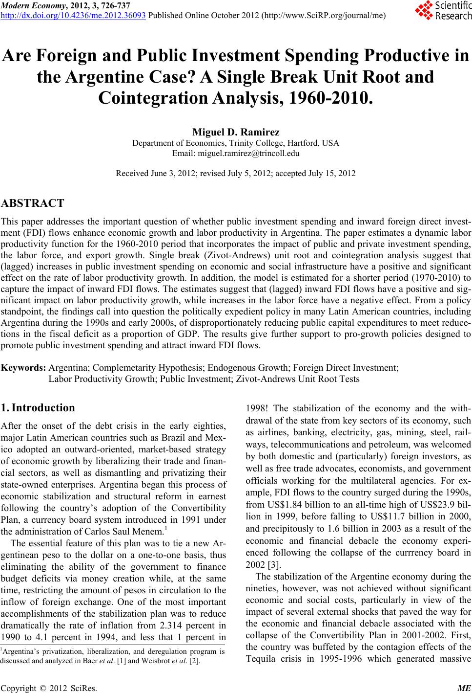
Modern Economy, 2012, 3, 726-737
http://dx.doi.org/10.4236/me.2012.36093 Published Online October 2012 (http://www.SciRP.org/journal/me)
Are Foreign and Public Investment Spending Productive in
the Argentine Case? A Single Break Unit Root and
Cointegration Analysis, 1960-2010.
Miguel D. Ramirez
Department of Economics, Trinity College, Hartford, USA
Received June 3, 2012; revised July 5, 2012; accepted July 15, 2012
ABSTRACT
This paper addresses the important question of whether public investment spending and inward foreign direct invest-
ment (FDI) flows enhance economic growth and labor productivity in Argentina. The paper estimates a dynamic labor
productivity function for the 1960-2010 period that incorporates the impact of public and private investment spending,
the labor force, and export growth. Single break (Zivot-Andrews) unit root and cointegration analysis suggest that
(lagged) increases in public investment spending on economic and social infrastructure have a positive and significant
effect on the rate of labor productivity growth. In addition, the model is estimated for a shorter period (1970-2010) to
capture the impact of inward FDI flows. The estimates suggest that (lagged) inward FDI flows have a positive and sig-
nificant impact on labor productivity growth, while increases in the labor force have a negative effect. From a policy
standpoint, the findings call into question the politically expedient policy in many Latin American countries, including
Argentina during the 1990s and early 2000s, of disproportionately reducing public capital expenditures to meet reduce-
tions in the fiscal deficit as a proportion of GDP. The results give further support to pro-growth policies designed to
promote public investment spending and attract inward FDI flows.
Keywords: Argentina; Complemetarity Hypothesis; Endogenous Growth; Foreign Direct Investment;
Labor Productivity Growth; Public Investment; Zivot-Andrews Unit Root Tests
1. Introduction
After the onset of the debt crisis in the early eighties,
major Latin American countries such as Brazil and Mex-
ico adopted an outward-oriented, market-based strategy
of economic growth by liberalizing their trade and finan-
cial sectors, as well as dismantling and privatizing their
state-owned enterprises. Argentina began this process of
economic stabilization and structural reform in earnest
following the country’s adoption of the Convertibility
Plan, a currency board system introduced in 1991 under
the administration of Carlos Saul Menem.1
The essential feature of this plan was to tie a new Ar-
gentinean peso to the dollar on a one-to-one basis, thus
eliminating the ability of the government to finance
budget deficits via money creation while, at the same
time, restricting the amount of pesos in circulation to the
inflow of foreign exchange. One of the most important
accomplishments of the stabilization plan was to reduce
dramatically the rate of inflation from 2.314 percent in
1990 to 4.1 percent in 1994, and less that 1 percent in
1998! The stabilization of the economy and the with-
drawal of the state from key sectors of its economy, such
as airlines, banking, electricity, gas, mining, steel, rail-
ways, telecommunications and petroleum, was welcomed
by both domestic and (particularly) foreign investors, as
well as free trade advocates, economists, and government
officials working for the multilateral agencies. For ex-
ample, FDI flows to the country surged during the 1990s,
from US$1.84 billion to an all-time high of US$23.9 bil-
lion in 1999, before falling to US$11.7 billion in 2000,
and precipitously to 1.6 billion in 2003 as a result of the
economic and financial debacle the economy experi-
enced following the collapse of the currrency board in
2002 [3].
The stabilization of the Argentine economy during the
nineties, however, was not achieved without significant
economic and social costs, particularly in view of the
impact of several external shocks that paved the way for
the economic and financial debacle associated with the
collapse of the Convertibility Plan in 2001-2002. First,
the country was buffeted by the contagion effects of the
Tequila crisis in 1995-1996 which generated massive
1Argentina’s privatization, liberalization, and deregulation program is
discussed and analyzed in Baer et al. [1] and Weisbrot et al. [2].
C
opyright © 2012 SciRes. ME

M. D. RAMIREZ 727
capital flight, a liquidity crisis, and high real interest rates
with their knock-on effects on the balance sheets of the
banks and the real economy. Second, the Asian and Rus-
sian crises led to a significant flight of capital and, once
again, a substantial rise in real interest rates and their
adverse effects. Third, the devaluation of the Brazilian
currency (the real) in 1999 had a severe effect on the
Argentine economy because close to 30 percent of its
exports were destined to that country (see [2]). This de-
velopment is all the more significant in view of the fact
that the government’s promotion of outward-oriented
policies has significantly increased the relative impor-
tance of its exports in fueling economic growth as at-
tested by the following figures: exports of goods and
services averaged 9.4 percent of GDP during the 1990-
2001 period as compared to 8.6 percent during the 1980-
1990 period [4]. Finally, the economic situation was fur-
ther exacerbated by the fact that the dollar continued to
appreciate in real terms relative to the Euro and the Yen,
thus further undermining the competitiveness of the Ar-
gentine economy given its hard peg to the dollar and its
policy of unrestricted mobility of capital (see [1]).
In addition to these external shocks, several prominent
investigators have focused on the long-term economic
(negative) effects associated with the severe IMF-spon-
sored stabilization and adjustment measures implemented
by the Argentine government, as well as other countries
in Latin America and the Caribbean (see [5-10]). These
programs often call for across-the-board cuts in public
spending and tight restrictions on credit creation in order
to meet stringent fiscal deficit targets, reduce the rate of
inflation, and free resources to service the external debt.2
In practice, critics contend that these stabilization and
adjustment measures further undermine investor and con-
sumer confidence because of their contractionary effect
on the real economy and the rate of capital formation.
Nowhere is this more evident than in the disappointing
and erratic behavior of Argentine private capital forma-
tion during the past two and a half decades. Table 1 be-
low shows that Argentina’s private investment as a pro-
portion of GDP fell dramatically during the lost decade
of the 1980s, reaching a low of 9.4 percent in 1990 which
amounted to less than half its level in 1980. Following
the adoption of the Convertibility Plan it rose to a high of
19.1 percent in 1994, from which it fell again to 9.2 per-
cent in 2002 and a dismal 7.6 percent in 2003 as a result
of the country’s economic crisis following the collapse of
the currency board. What is particularly worrisome about
these figures is that most economists believe that it is
absolutely essential for Argentina—and other countries
Table 1. Argentina: Investment as a share of GDP (in per-
cent), 1980-2010.
Year Private Investment Public Investment
1980 19.2 6.1
1982 16.6 5.2
1984 14.9 5.0
1986 13.2 4.3
1988 14.4 4.3
1990 9.4 4.6
1992 14.9 1.8
1994 19.1 0.8
1996 16.1 2.0
1998 17.9 2.0
2000 15.4 1.0
2001 12.1 0.9
2002 9.2 0.7
2003 7.6 0.8
2004 10.5 1.3
2005 12.9 1.9
2006 13.2 2.5
2007 14.8 3.3
2008 15.1 3.3
2009 13.5 3.5
2010 14.9 3.5
Average
1970-1979 13.6 9.1
1980-1989 15.0 4.9
1990-1999 15.7 1.6
2000-2010 12.7 2.1
Source: IFC, Trends in Private Investment in Developing Countries, Statis-
tics for 1970-2000. Washington DC, The World Bank, 2001; M.E.P., Ar-
gentina: Sustainable Output Growth After the Collapse. Buenos Aires, Min-
isterio De Economia Argentina, 2003, Tables 1 and 2 pp. 7-11; and ECLAC
(2010).
of Latin America—to significantly improve and sustain
its investment performance if it is going to lay the
groundwork for rapid and sustained economic growth, as
well as create future employment opportunities for its
rapidly expanding labor force (see [10]).
A number of investigators have cited the dramatic fall
in public investment in economic and social infrastruc-
ture, brought about by the need to meet the stringent fis-
cal deficit targets of the stabilization program, as one
2Weisbrot et. al. ([2]: p. 3) reports that in 2002 the IMF demanded that
the Argentine government enact spending cuts of 10 percent across-
the-board, in addition to a 30 percent reduction in outlays for goods and
services and a 13 percent cut in salary and pensions for government
employees.

M. D. RAMIREZ 728
possible factor in explaining the poor investment per-
formance of Argentina and other Latin American coun-
tries. Table 1 shows that public investment spending in
economic and social infrastructure as a proportion of
GDP fell precipitously from 4.6 percent in 1990 to barely
1 percent in 1994, only to rise to 2 percent during the
1995-1999 period before falling again in the 2001-2003
period to less than 1 percent. Moreover, the average pub-
lic investment spending on economic infrastructure for
the 1990s and early 2000s is only a third of that of the
1980s and barely one fifth of the average level recorded
during the 1970s. However, Table 1 also reveals that
under the pro-growth policies of the Kirschner admini-
stration (2003-2010) public investment as percentage of
GDP has risen dramatically since 2005, recording levels
well above 3 percent since 2007.
The basic idea is that public investments in highways,
bridges, sewerage systems, water supplies, and education
and health services often generate substantial positive
spillover benefits for the private sector by reducing the
direct (and indirect) costs of producing, transporting, and
delivering goods and services to consumers (see [11-14]).
If the complementarity hypothesis is correct, then the
steep reductions in public capital formation experienced
in Argentina and elsewhere in Latin America during the
past decade and a half may further depress private in-
vestment spending and productivity growth. Moreover, it
may also undermine some or all of the long-term effi-
ciency gains anticipated from the implementation of
market-based, outward-oriented reforms such as privati-
zation of state-owned firms and the liberalization of trade
and finance (see [15]). After all, the newly privatized
firms in liberalized (open) markets will need adequate
and reliable economic infrastructure in order to produce,
transport, and market their goods and services at home
and abroad in a cost-effective manner.
In view of the importance and controversial nature of
this topic, this paper analyzes the impact of public in-
vestment spending, inward FDI flows, and export growth
on the economic growth and labor productivity of the
Argentine economy. The choice of Argentina is war-
ranted for a number of reasons. First, Argentina is a large
and strategically important country in Latin America.
This is a situation that promises to continue as a result of
the country’s participation in the important regional trade
agreement named Mercosur. Second, beginning with the
Menem administration (1989-1999) and continuing under
the ill-fated administrations of Fernando De La Rua and
Duhalde (2000-2002), Argentina pursued a far-reaching
market-based strategy of economic growth and develop-
ment, while under both Kirschner administrations (2003-
2010), the Argentine government has reversed itself and
pursued a more activist set of growth policies.3 An
econometric study of the impact of public investment
spending, FDI inflows, and export growth in a major
Latin American nation under these different regimes
should prove both interesting and useful to development
scholars and policymakers as they decide where to allo-
cate scarce public funds to maximize the country’s
growth potential. Finally, Argentina is one of the few
countries in Latin America that has reliable and disag-
gregated time-series data on public investment spending
on economic and social infrastructure going as far back
as the decade of the sixties. This data set thus enables
researchers to test whether increases in government in-
vestment spending on economic infrastructure per se,
rather than overall public investment expenditures, dis-
place or promote private investment spending, economic
growth, and (labor) productivity.
The paper is organized as follows. Section 2 provides
a conceptual framework for incorporating the public or
FDI capital stock in a modified neoclassical production
function. The model presented in this section is intended
solely to motivate the ensuing discussion and although
the relevant parameters cannot be estimated directly
given the inherent data limitations present in the Argen-
tine case, the discussion highlights how researchers
might proceed if the relevant data becomes available.
Next, the paper introduces a rough empirical counterpart
to the model presented in the previous section, and dis-
cusses the nature and limitations of the data used in this
study. Section 4 presents single break (Zivot-Andrews)
unit root tests and the estimates for the dynamic produc-
tion relationship. Using cointegration analysis, this sec-
tion tests whether there is a stable long-term relationship
among the relevant regressors of the modified production
function. In so doing, this paper goes beyond other em-
pirical studies of the complementarity hypothesis by ad-
dressing the important question of spurious correlation
among the model variables. The section is brought to a
close by generating several error-correction (EC) models
that are used to track the historical data on the growth
rate of output for the period under review. The last sec-
tion summarizes the paper’s major findings.
2. The Model
On the supply side, the positive externalities generated
by additions to the public (or FDI) capital stock can be
formalized by incorporating them in an augmented
Cobb-Douglas production function of the following form
3Under both Kirschner administrations, the economy has grown at
average annual rates exceeding 8 percent and levels of poverty and
unemployment have experienced a dramatic fall from their crisis levels
in 2001-2002; there has also been a huge increase in government
spending on housing, health, and economic infrastructure, as well as a
significant extension of social security coverage and a substantial rise
in real wages (see [16]: pp. 8-12).

M. D. RAMIREZ 729
[17]:

1
ALKE

,,
p
YALKE



,,
pg
ELKK

 
 (1)
where Y is real output, Kp is the private capital stock, L is
labor, and E denotes the externality generated by addi-
tions of the public capital stock or FDI capital stock (α
and β are the shares of domestic labor and private capital
respectively, and A captures the efficiency of production.
Initially, it is assumed that α and β are less than one, such
that there are diminishing returns to the labor and capital
inputs.
The externality, E, can be represented by a Cobb-
Douglas function of the type:





1
pg
K
 (2)
where γ and θ are, respectively, the marginal and the in-
tertemporal elasticities of substitution between private
and public (FDI) capital. Let γ > 0, such that a larger
stock of public (or FDI) capital generates a positive ex-
ternality to the economy. If θ > 0, intertemporal com-
plementarity prevails and, if θ < 0, additions to stock of
public (FDI) capital crowd out private capital over time
(see [18]).
Combining Equations (1) and (2), we obtain,

11
YAL K


   

   



(3)
A standard growth accounting equation can be derived
by taking logarithms and time derivatives of Equation (3)
to generate the following dynamic production function:
1
1
1
y
AL
Kp
Kg
g
gg
g
g


 



 




pt
t eLtdt


11

 
 

 


(4)
where gi is the growth rate of i = Y, A, L, Kp, and Kg.
Equation (4) states that (provided γ and θ > 0) additions
to the stock of public (FDI) capital will augment the elas-
ticities of output with respect to labor and capital by a
factor θ(1 – α – β).
The demand side of the economy can be included into
the model via the following intertemporal utility maxi-
mization framework:

max o ut uc

 (5)
s.t.

p
pg p
K
AK K
 
c k


 
 , and


00
p
K
  
.
where, for convenience, lower-case letters are defined in
per capita terms and ρ is the discount rate, L(t) is the size
of the family, c(t) is per capita consumption, and δ
represents the rate of depreciation. For convenience, the
initial population is normalized to 1 so that the analysis
in aggregate and per capita terms is the same. The in-
stantaneous utility function of the representative con-
sumer is assumed to exhibit constant relative risk and can
be written in the following general form:



111uct ct  



(6)
σ denotes the relative risk aversion coefficient or the in-
verse of the elasticity of substitution between current and
future consumption; i.e., σ is an index of the representa-
tive consumer’s willingness to exchange current con-
sumption for future consumption. Letting u(c) = lnc, for
simplicity, and solving the standard optimal control
problem in Equation (5), we obtain the following equa-
tion:


 

11 1
11
pg
cc AKK
 
 



 

 (7)
Equation (7) can be interpreted as follows in the pre-
sence of intertemporal complementarity between public
(FDI) and private capital (i.e., θ > 0): the economy grows
at a positive rate whenever the marginal product of capi-
tal, net of depreciation, can be kept above the rate of time
preference (discount). The marginal productivity of pri-
vate capital, in turn, is augmented and kept above the
discount rate by additions to the stock of public (or FDI)
capital. Finally, the larger the intertemporal elasticity of
substitution of current consumption for future consump-
tion, as captured by the inverse of the relative risk coeffi-
cient, σ, the higher the rate of growth of the economy.
Put differently, the sacrifice of current consumption is
less costly to the representative consumer when present
and future consumption are good substitutes
3. Empirical Model
In the development literature it is often not possible to
generate estimates of Equations (3) and (4) above be-
cause of the poor quality of existing data for public and
private investment spending, as well as the actual paucity
of data on the labor force over a sufficiently long period
of time. Instead, investigators have used proxies for key
variables such as the labor force and/or the stocks of pri-
vate and public capital such as population data rather
than labor force data, or substituted investment data (as a
proportion of GDP) for capital stock data (see [19,20]).
Alexander [21] has shown, however, that models using
these proxies have to impose unduly restrictive assump-
tions (e.g., such as a fixed capital-output ratio) or unreal-
istic assumptions (a constant labor force participation
rate) that can generate both misspecified relationships
and significant measurement errors.
In the case of Argentina we are fortunate to have labor
force data going as far back as 1960, but we do not have
consistent estimates of the public and private capital
stock series, or for that matter, reliable estimates of the
rate of depreciation from which such a series could be

M. D. RAMIREZ 730
generated. Researchers in the field of economic deve-
lopment have circumvented this problem by estimating a
dynamic production which defines the relevant variables
in terms of percentage growth rates, thus permitting them
to generate proxies for the percentage growth rates in the
respective capital stocks. Following their lead, this study
includes the ratio of public and private investment spend-
ing to gross domestic product as alternative proxies. Fi-
nally, for reasons explained in Section IV, the empirical
model was estimated with changes in the investment ra-
tios because these ratios were determined to be nonsta-
tionary in level form. This study thus extends previous
empirical work by estimating a rough empirical counter-
part of the dynamic production function in Equation (4)
for the 1960-2010 period without the FDI variable and
between 1970 and 2010 with the FDI variable.4
The most general formulation of the growth equation
is given below,



12 3
567
 
4
182
p
gf
ii
DD



 
g
yli
cx
 

 
 (8)
lower case letters denote natural logarithms, and Δ de-
notes the change in the variable in question; y is real
GDP (1993 pesos); l, as indicated above, refers to the
labor force (thousands occupied); ip denotes the ratio of
private investment to GDP, while ig represents public
investment spending on economic and social infrastruc-
ture as a proportion of GDP, viz., roads, bridges, and
education5—it therefore excludes investment expendi-
tures by state-owned enterprises which are more likely to
crowd out private investment spending and output; if the
ratio of foreign direct investment to GDP and it is ex-
pected to have a positive effect because increased FDI
flows are associated with a greater transfer of technology
and managerial knowhow, learning-by-doing, and greater
market discipline; however, FDI flows may also have a
negative effect on the growth rate of a country if they
give rise to substantial reverse flows in the form of re-
mittances of profits and dividends and/or if the TNCs
obtain substantial tax and other concessions from the
host country (see [22]); cg is real government consump-
tion expenditures as a proportion of GDP, and may di-
rectly or indirectly (via output taxes) crowd out private
expenditures and thus affect output in a negative fashion;
x denotes exports of goods and services and, as suggested
by the export promotion hypothesis, its growth rate is
expected not only to have a direct effect on economic
growth, but also indirectly via the increased investment
and realization of economies of scale by the exporting
firms, and the concomitant diffusion of technological and
managerial knowhow throughout the economy generated
by the export sector; D1 is a dummy variable that takes a
value of one for the crisis years, and 0 otherwise, while
D2 equals 1 for the impact of the currency board, and 0
otherwise.
Data
The data used in this study were obtained from official
government sources such as the Direccion Nacional de
Politicas Macroeconomica, Ministerio de Economia y
Produccion (Ministry of Economy and Production, vari-
ous issues) and the Instituto Nacional De Estadistica y
Censos de la Republica Argentina (National Institute of
Statistics and Census of Argentina). Other relevant eco-
nomic data have been obtained from ECLAC, Statistical
Yearbook for Latin America and the Caribbean, 2010,
and the International Finance Corporation [23].
In this study we focused on labor productivity so the
dependent variable was estimated as the growth rate in
labor productivity by subtracting the growth rate in the
labor force from the percentage change in GDP in Equa-
tion (8). Defining the dependent variable in this manner
reverses the expected sign of the labor variable because
of diminishing returns to the labor input. The sign of β1 is
anticipated to be positive in the GDP formulation while,
as indicated above, it is expected to be negative in the
labor productivity specification. β2 is expected to be
positive, while the sign of β3 can be positive or negative
depending on whether increases in public in public in-
vestment complement or substitute for private capital
formation. Lags were included for this variable to ad-
dress both the delayed impact of government investment
spending on private output growth, as well as reverse
causation.6
The sign of β4 is also indeterminate because govern-
ment expenditures on collective consumption goods such
as food, housing, and salaries of public employees may
directly or indirectly (via output taxes and subsidies)
crowd out private consumption expenditures and thus
6To test for reverse causality, a Granger-causality test was performed
with four lags. The results show that the null hypothesis that private
investment does not “Granger cause” real GDP (labor productivity) can
be rejected at the 5 percent level (p-value: 0.04), but not the other way
around (p-value: 0.07). Similarly, the null that government investment
does not “Granger cause” real GDP (labor productivity) is strongly
rejected at the 5 percent level (p-value: 0.01), but not the other way
around (p-value: 0.82). In the case of the labor force the null can only
be rejected at the 10 percent level, while it cannot be rejected in the
reverse direction (p-value: 0.31); finally, in the case of the export vari-
able the null cannot be rejected in either direction (p-values: 0.13 and
0.15, respectively). Of course, this test says nothing about “causation”
p
e
r
se, it only provides information about whether changes in one vari-
able precede changes in another.
4Data for the FDI ratio were not available for Argentina prior to 1970
[6].
5Government investment data (and government consumption data)
contains a portion that is devoted to health and education expenditures,
and should be treated separately as public (human) capital investment.
However, to my knowledge, there are no disaggregated government
expenditures on education or enrollment ratios for the period under
review which I could use as proxies for the human capital variable.

M. D. RAMIREZ 731
affect output in a negative fashion. β5 is expected to have
a positive sign, but for reasons alluded to above, its sign
could also be negative. β6 is expected to be positive for
reasons alluded to above, while β7 is anticipated to be
negative for obvious reasons; finally, β8 is expected to be
positive.
4. Unit Roots, Structural Breaks, and
Cointegration Analysis
Initially, conventional unit root tests (without a structural
break) were undertaken for the variables in question
given that it is well-known that macro time series data
tend to exhibit a deterministic and/or stochastic trend that
renders them non-stationary; i.e., the variables have
means, variances, and covariances that are not time in-
variant (see [24])). This study tested the variables in
question for a unit root (non-stationarity) by using an
Augmented Dickey-Fuller test (ADF) with a lag length
automatically determined by the Schwarz Information
Criterion (SIC).
Before reporting the unit root tests, it is important to
acknowledge that when dealing with historical time se-
ries data for developing countries such as Argentina or
Chile investigators are often constrained by the relatively
small number of time series observations (usually in an-
nual terms). This is the case in this study where the sam-
ple size is just at the threshold level of 50 observations
recommended by Granger and Newbold [25], which may
compromise the power of the unit root (and cointegration)
tests—not to mention distort the size or significance of
the tests as well (see [26]). However, a growing literature
contends that the power of unit root (and cointegration)
tests depends on the length or time span of the data more
than the mere number of observations in the sample. That
is, for a given sample size n, the power of the test is
greater when the time span is large. Thus, unit root or
cointegration tests based on 45 observations over 45
years have considerable more power than those based on
100 observations over 100 days (see [27,28]).7
Table 2 presents the results of running an ADF test
(one lag) for the variables in both level and differenced
form under the assumption of a stochastic trend only, i.e.,
the test is run with a constant term and no time trend. It
can be readily seen that all the variables in level form are
nonstationary; i.e., they appear to follow a random walk
with (positive) drift. In the case of first differences,
Table 2. Argentina: Unit root tests for stationarity, sample
period 1960-2010.
Variables LevelsFirst
Difference
5% Critical
Value1
1% Critical
Value
ln(Y) –0.15 –5.39** –2.92 –3.57
ln(Y/L) –2.15 –5.07** –2.92 –3.57
lnL 1.30 –6.19** –2.92 –3.57
lnIp –1.54 –5.64** –2.92 –3.57
lnIg –1.52 –6.34** –2.92 –3.57
lnCg –1.66 –4.19** –2.92 –3.57
lnIf2 –2.51 –6.67** –2.92 –3.57
lnX –0.64 –6.89** –2.92 –3.57
1MacKinnon critical values for rejection of hypothesis of a unit root. 2Unit
root tests for the FDI variable were undertaken for the 1970-2010 period.
*Denotes significant at the 5 percent level; **denotes significance at the 1
percent level. Estimations undertaken with Eviews 7.2.
however, the null hypothesis of non-stationarity is re-
jected for all variables (except one) at least at the 5 per-
cent level. Thus, the evidence presented suggests that the
variables in question follow primarily a stochastic trend
as opposed to a deterministic one, although the possibil-
ity that for given subperiods they follow a mixed process
cannot be rejected.
Although suggestive, the conventional results reported
in Table 2 may be misleading because the power of the
ADF test may be significantly reduced when the station-
ary alternative is true and a structural break is ignored
(see [29]); that is, the investigator may erroneously con-
clude that there is a unit root in the relevant series. In
order to test for an unknown one-time break in the data,
Zivot and Andrews [29] developed a data dependent al-
gorithm that regards each data point as a potential break-
date and runs a regression for every possible break-date
sequentially. The test involves running three regressions
(models): model A which allows for a one-time change in
the intercept of the series; model B which permits a
one-time change in the slope of the trend function; and
model C which combines a one-time structural break in
the intercept and trend [30]. Following the lead of Perron,
most investigators report estimates for either models A
and C, but in a relatively recent study Sen [31] has
shown that the loss in test power (1 – β) is considerable
when the correct model is C and researchers erroneously
assume that the break-point occurs according to model A.
On the other hand, the loss of power is minimal if the
break date is correctly characterized by model A but in-
vestigators erroneously use model C. In view of this,
Table 3 reports the Zivot-Andrews (Z-A) one-break unit
root test results for model C in level form along with the
endogenously determined one-time break date for each
time series.
7Hakkio and Rush ([28]: p. 579) contend that in nearly non-stationary
time series “the frequency of observation plays a very minor role” in
cointegration [and unit root] analysis because “cointegration is a long-
run property, and thus we often need long spans of data to properly test
it”. Similarly, Bahmani-Oskooee ([27]: p. 481) observes that in cointe-
gration (and unit root) analysis using ann ual data over 30 years “is as
good as using quarterly data over the same period”. To some degree,
this addresses the strong analytical and policy inferences drawn from a
relatively small sample size.

M. D. RAMIREZ 732
Table 3. Zivot-Andrews one-break unit root test, sample
period 1960-2010.
Variables Levels Break Year5% Critical
Value
1% Critical
Value
Ln(Y) –3.37 1980 –5.08 –5.57
In(Y/L) –2.96 1980 –5.08 –5.57
lnL –4.36 2000 –5.08 –5.57
lnIp –4.43 1979 –5.08 –5.57
lnIg –3.28 1991 –5.08 -5.57
lnCg –2.69 1980 –5.08 –5.57
lnIf –4.38 1995 –5.08 –5.57
lnX –4.08 1973 –5.08 –5.57
Estimations undertaken with Eviews 7.2.
As can be readily seen, the estimates reported in Table
3 for the series in level form are consistent with those in
Table 2. For all of the series in question, Table 3 shows
that the null hypothesis with a structural break in both the
intercept and the trend cannot be rejected at the 5 percent
level of significance. In addition, the Z-A test identifies
endogenously the single most significant structural break
in every time series. In view of space constraints, Figure
1 below shows the endogenously determined break-date
for the labor productivity (lprod) series.8
Having shown that the variables are integrated of order
one, I(1), it is necessary to determine whether there is at
least one linear combination of these variables that is I(0).
In other words, does there exist a stable and non-spurious
(cointegrated) relationship among the regressors in each
of the relevant specifications? This was done by using
the cointegration method proposed by Johansen and
Juselius [33]. The Johansen method was chosen over the
one originally proposed by Engle and Granger [25] be-
cause it is capable of determining the number of cointe-
grating vectors for any given number of non-stationary
series (of the same order), its application is appropriate in
the presence of more than two variables, and more im-
portant, the likehood ratio tests used in the procedure
(unlike the ADF tests) have well- defined limiting distri-
butions (see [34]).
Table 4 below shows that the Johansen test for both
the output and labor productivity equations show that the
null hypothesis of no cointegrating vector can be rejected
at least at the one percent level; i.e., there exists a unique
linear combination of the I(1) variables that links them in
a stable and long-run relationship.9 The signs of the
Zivot-Andrews unit root test
Date: 06/01/12 Time: 15:06
Sample: 1960-2010
Included observations: 51
Null hypothesis: LPROD has a unit root with a structural
Break in both the intercept and trend
Chosen lag length: 1 (maximum lags: 4)
Chosen break point: 1980
t-Statistic Prob.*
Zivot-Andrews test statistic –2.958391 0.117365
1% critical value: –5.57
5% critical value: –5.08
10% critical value: –4.82
* Probability values are calculated from a standard t-distribution.
Figure 1. Break-date for labor productivity series.
cointegrating equation are reversed because of the nor-
malization process and they suggest that, in the long run,
the private and government investment variables have a
positive and highly significant effect on Argentine labor
productivity. The relatively high private capital (invest-
ment) elasticity reported in Table 4 is consistent with the
extant empirical literature for developing (and developed)
countries, and may be explained by FDI-induced or edu-
cational externalities in the form of better managerial
know-how and the transfer of superior technology that
“inflate” the private investment elasticity estimate by a
positive factor θ (see [17]). For example, a Ceteris pari-
bus 10 percent increase in the ratio of private investment
to GDP raises output per worker by an estimated 5.6
percent in the long run. Admittedly, the relatively high
coefficient for the labor variable may also be due to
measurement error, omitted variables such as human
capital, and/or simultaneity bias.
8In a relatively recent paper, Lee and Stazicich [32] show that when
there are, in fact, two structural breaks in the data, assuming errone-
ously that there is only one can result in a loss of power of the test.
9Dummy variables were treated as exogenous variables in the cointe-
gration test. The variables in question are also cointegrated with the
inclusion of the export variable. There is only one unique cointegrating
vector. The Max-eigenvalue test also reveals one cointegrating vector
at the 5 percent level.

M. D. RAMIREZ 733
Table 4. Johansen cointegration rank test (Trace), 1960-
2010.
A. Series: lnY, lnL, LnIg, and lnIp.
Test assumption: No Linear deterministic trend in the data.
Eigenvalue Likelihood Ratio 5% Critical Value No. of CE(s)
0.490 58.293 54.08 None
0.330 25.291 35.19 At most 1
0.088 5.633 20.26 At most 2
0.022 1.132 9.17 At most 3
B. Series: ln(Y/L), lnL, lnIg, and lnIp.
Test assumption: No linear deterministic trend in the data.
Eigenvalue Likelihood Ratio 5% Critical Value No. of CE(s)
0.534 66.786 54.08 None
0.363 30.193 35.19 At most 1
0.128 8.477 20.26 At most 2
0.039 1.912 9.17 At most 3
Normalized cointegrating vector;
coefficients normalized on ln(Y/L) in parenthesis.
Vector ln(Y/L) lnL lnIg lnIp Constant
1. 1.000 1.217 –0.557 –0.082 –4.407
(0.627) (0.104) (0.026)
Note: Standard errors are in parenthesis. Estimation undertaken with Eviews
7.2.
The lagged residual (error correction (EC) term) from
the cointegrating equation, measuring the deviation be-
tween the current level of output (labor productivity) and
the level based on the long-run relationship, was included
in a set of EC models. For simplicity, consider the EC
model without lags (and dummy variables) given in
Equation (6) below:
 


12 3
56
EC
 
4
1
p
gg
ic 



ft
yli
ix
 


 
 (9)
The coefficients (β = s) of the changes in the relevant
variables represent short-run elasticities, while the coef-
ficient, δ (< 0), on the lagged EC term obtained from the
cointegrating equation in level form denotes the speed of
adjustment back to the long-run relationship among the
variables. To conserve space, Table 5 below presents
results only for the labor productivity growth rate rela-
tionship. The results for Equations (1)-(3) (for the longer
time period without the FDI variable but with the inclu-
sion of the export variable) suggest that the immediate
impact of changes in the growth rate of the private in-
vestment ratio is positive and statistically (and economi-
Table 5. Argentina: Error correction model; Dependent
variable is: (ΔlnYt - ΔlnLt), 1960-2010.
OLS Regressions
Variables(1) (2) (3) (4) (5)
Constant 0.01 0.01 0.01 0.02 0.08
(1.10) (1.20) (1.55)* (1.91)*(1.94)*
ΔlnLt–1 –0.42 –0.31 –0.43 –0.21 –0.23
(–3.69)** (–2.10)** (–3.26)* (–1.30)(–1.34)
Δln(Ip/Y)t–1 0.07 0.08 0.07 0.12 0.11
(2.36)** (5.56)** (2.36)** (3.68)**(4.36)**
Δln(Ig/Y)t–2 0.02 0.02 0.02 0.03 0.02
(2.82)** (1.94)** (3.22)** (2.15)**(2.12)**
Δln(If/Y)t–3 --- --- --- 0.01 0.01
(3.36)**(2.77)**
ΔlnXt–1 0.05 0.06 0.06 --- ---
(2.26)** (2.21)** (2.22)**
Δln(C/Y)t–1 --- –0.01 --- --- ---
(1.13)
ECTt–1 –0.18 –0.19 –0.15 –0.17 –0.11
(–2.20)** (–3.15)** (–2.20)** (–2.17)** (–2.33)**
DUM1 --- –0.03 –0.04 --- –0.04
(–2.38)** (–4.66)** (–4.07)**
DUM2 --- --- 0.03 --- ---
(4.52)**
Adj R2 0.64 0.70 0.73 0.70 0.75
S.E. 0.026 0.029 0.026 0.028 0.021
D.W. 1.88 2.09 2.05 1.90 2.02
Ramsey
Test (p:0.26) (p:0.71) (p:0.87) (p:0.33) (p:0.97)
AIC –4.26 –4.06 –4.30 –3.91 –4.02
SIC –3.89 –4.78 –3.92 –3.46 –3.53
Note: Figures in parentheses are t-ratios; asterisks denotes significance as
follows: *at the 10 percent level and **at least at the 5 percent level. AIC
denotes Akaike Information Criterion and SIC is the Schwarz Information
Criterion.
cally) significant, while lagged changes in employment
growth have an (expected) negative impact on the growth
rate in labor productivity. Turning to the public invest-
ment variable, it can be readily seen that this variable has
a positive and statistically significant effect when lagged
one to two periods. This result is not altogether surpris-
ing because the positive externalities generated from ad-
ditions to the stock of roads, bridges and ports are likely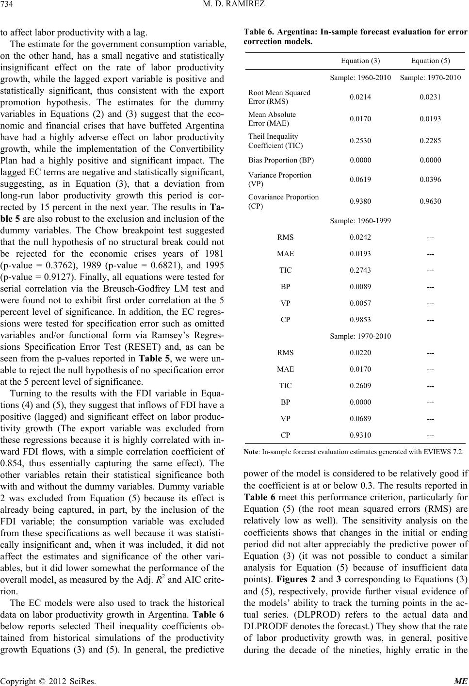

M. D. RAMIREZ 734
to affect labor productivity with a lag.
The estimate for the government consumption variable,
on the other hand, has a small negative and statistically
insignificant effect on the rate of labor productivity
growth, while the lagged export variable is positive and
statistically significant, thus consistent with the export
promotion hypothesis. The estimates for the dummy
variables in Equations (2) and (3) suggest that the eco-
nomic and financial crises that have buffeted Argentina
have had a highly adverse effect on labor productivity
growth, while the implementation of the Convertibility
Plan had a highly positive and significant impact. The
lagged EC terms are negative and statistically significant,
suggesting, as in Equation (3), that a deviation from
long-run labor productivity growth this period is cor-
rected by 15 percent in the next year. The results in Ta-
ble 5 are also robust to the exclusion and inclusion of the
dummy variables. The Chow breakpoint test suggested
that the null hypothesis of no structural break could not
be rejected for the economic crises years of 1981
(p-value = 0.3762), 1989 (p-value = 0.6821), and 1995
(p-value = 0.9127). Finally, all equations were tested for
serial correlation via the Breusch-Godfrey LM test and
were found not to exhibit first order correlation at the 5
percent level of significance. In addition, the EC regres-
sions were tested for specification error such as omitted
variables and/or functional form via Ramsey’s Regres-
sions Specification Error Test (RESET) and, as can be
seen from the p-values reported in Table 5, we were un-
able to reject the null hypothesis of no specification error
at the 5 percent level of significance.
Turning to the results with the FDI variable in Equa-
tions (4) and (5), they suggest that inflows of FDI have a
positive (lagged) and significant effect on labor produc-
tivity growth (The export variable was excluded from
these regressions because it is highly correlated with in-
ward FDI flows, with a simple correlation coefficient of
0.854, thus essentially capturing the same effect). The
other variables retain their statistical significance both
with and without the dummy variables. Dummy variable
2 was excluded from Equation (5) because its effect is
already being captured, in part, by the inclusion of the
FDI variable; the consumption variable was excluded
from these specifications as well because it was statisti-
cally insignificant and, when it was included, it did not
affect the estimates and significance of the other vari-
ables, but it did lower somewhat the performance of the
overall model, as measured by the Adj. R2 and AIC crite-
rion.
The EC models were also used to track the historical
data on labor productivity growth in Argentina. Table 6
below reports selected Theil inequality coefficients ob-
tained from historical simulations of the productivity
growth Equations (3) and (5). In general, the predictive
Table 6. Argentina: In-sample forecast evaluation for error
correction models.
Equation (3) Equation (5)
Sample: 1960-2010 Sample: 1970-2010
Root Mean Squared
Error (RMS) 0.0214 0.0231
Mean Absolute
Error (MAE) 0.0170 0.0193
Theil Inequality
Coefficient (TIC) 0.2530 0.2285
Bias Proportion (BP) 0.0000 0.0000
Variance Proportion
(VP) 0.0619 0.0396
Covariance Proportion
(CP) 0.9380 0.9630
Sample: 1960-1999
RMS 0.0242 ---
MAE 0.0193 ---
TIC 0.2743 ---
BP 0.0089 ---
VP 0.0057 ---
CP 0.9853 ---
Sample: 1970-2010
RMS 0.0220 ---
MAE 0.0170 ---
TIC 0.2609 ---
BP 0.0000 ---
VP 0.0689 ---
CP 0.9310 ---
Note: In-sample forecast evaluation estimates generated with EVIEWS 7.2.
power of the model is considered to be relatively good if
the coefficient is at or below 0.3. The results reported in
Table 6 meet this performance criterion, particularly for
Equation (5) (the root mean squared errors (RMS) are
relatively low as well). The sensitivity analysis on the
coefficients shows that changes in the initial or ending
period did not alter appreciably the predictive power of
Equation (3) (it was not possible to conduct a similar
analysis for Equation (5) because of insufficient data
points). Figures 2 and 3 corresponding to Equations (3)
and (5), respectively, provide further visual evidence of
the models’ ability to track the turning points in the ac-
tual series. (DLPROD) refers to the actual data and
DLPRODF denotes the forecast.) They show that the rate
of labor productivity growth was, in general, positive
during the decade of the nineties, highly erratic in the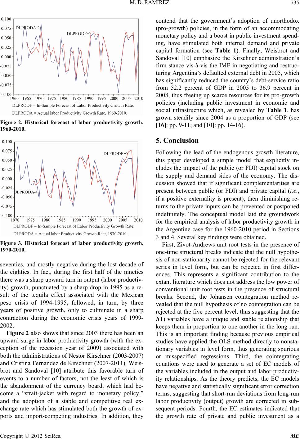

M. D. RAMIREZ 735
Figure 2. Historical forecast of labor productivity growth,
1960-2010.
Figure 3. Historical forecast of labor productivity growth,
1970-2010.
seventies, and mostly negative during the lost decade of
the eighties. In fact, during the first half of the nineties
there was a sharp upward turn in output (labor productiv-
ity) growth, punctuated by a sharp drop in 1995 as a re-
sult of the tequila effect associated with the Mexican
peso crisis of 1994-1995, followed, in turn, by three
years of positive growth, only to culminate in a sharp
contraction during the economic crisis years of 1999-
2002.
Figure 2 also shows that since 2003 there has been an
upward surge in labor productivity growth (with the ex-
ception of the recession year of 2009) associated with
both the administrations of Nestor Kirschner (2003-2007)
and Cristina Fernandez de Kirschner (2007-2011). Weis-
brot and Sandoval [10] attribute this favorable turn of
events to a number of factors, not the least of which is
the abandonment of the currency board, which had be-
come a “strait-jacket with regard to monetary policy,”
and the adoption of a stable and competitive real ex-
change rate which has stimulated both the growth of ex-
ports and import-competing industries. In addition, they
contend that the government’s adoption of unorthodox
(pro-growth) policies, in the form of an accommodating
monetary policy and a boost in public investment spend-
ing, have stimulated both internal demand and private
capital formation (see Table 1). Finally, Weisbrot and
Sandoval [10] emphasize the Kirschner administration’s
firm stance vis-à-vis the IMF in negotiating and restruc-
turing Argentina’s defaulted external debt in 2005, which
has significantly reduced the country’s debt-service ratio
from 52.2 percent of GDP in 2005 to 36.9 percent in
2008, thus freeing up scarce resources for its pro-growth
policies (including public investment in economic and
social infrastructure which, as revealed by Table 1, has
grown steadily since 2004 as a proportion of GDP (see
[16]: pp. 9-11; and [10]: pp. 14-16).
5. Conclusion
Following the lead of the endogenous growth literature,
this paper developed a simple model that explicitly in-
cludes the impact of the public (or FDI) capital stock on
the supply and demand sides of the economy. The dis-
cussion showed that if significant complementarities are
present between public (or FDI) and private capital (i.e.,
if a positive externality is present), then diminishing re-
turns to the private inputs can be prevented or postponed
indefinitely. The conceptual model laid the groundwork
for the empirical analysis of labor productivity growth in
the Argentine case for the 1960-2010 period in Sections
3 and 4. Several key findings were obtained.
First, Zivot-Andrews unit root tests in the presence of
one-time structural breaks indicate that the null hypothe-
sis of non-stationarity cannot be rejected for the relevant
series in level form, but can be rejected in first differ-
ences. This represents a significant contribution to the
extant literature which does not address the low power of
conventional unit root tests in the presence of structural
breaks. Second, the Johansen cointegration method re-
vealed that the null hypothesis of no cointegration can be
rejected at the five percent level, thus suggesting that the
I(1) variables have a unique and stable relationship that
keeps them in proportion to one another in the long run.
This is an important finding because previous empirical
studies have applied the OLS method directly to nonsta-
tionary variables in level form, thus generating spurious
or misspecified regressions. Third, the cointegrating
equations were used to generate a set of EC models of
the variables included in the output and labor productiv-
ity relationships. As the theory predicts, the EC models
have negative and statistically significant error correction
terms, suggesting that short-run deviations from long-run
labor productivity (output) growth are corrected in sub-
sequent periods. Fourth, the EC estimates indicated that
the growth rate of private and public investment as a

M. D. RAMIREZ 736
proportion of GDP, as well as the growth rate in exports
and the FDI ratio, have a positive and statistically sig-
nificant effect on the growth rate of labor productivity,
while the growth rate in the labor force has a negative
impact. Fifth, the reported Theil inequality coefficients
for the selected EC models suggested that they were able
to track and simulate the turning points of the historical
series in labor productivity relatively well.
Finally, the EC model estimates showed that during
the decade of the nineties the rate of labor productivity
growth was mostly positive, while during the decade of
the seventies the annual estimated rate of output growth
became erratic, culminating in a marked decrease (often
negative rates) during the decade of the eighties—the
so-called lost decade of development. The labor produc-
tivity growth estimates for the first half of the nineties
did reveal a robust increase, thereby suggesting that the
currency board’s taming of inflationary pressures and the
opening of the economy to foreign direct investment had
a positive effect. During the second half of the 2000s,
there has been an upsurge in labor productivity growth
which has coincided with the promotion by both Kir-
schner administrations of pro-growth policies, including
a significant increase in public investment as a propor-
tion of GDP which averaged 3 percent during the 2005-
2010 period—more than triple its average during the
2000-2004 interval.
From a policy standpoint, the findings in this paper are
important because they suggest that cash-strapped gov-
ernments of Latin America, such as the Argentine one,
can maximize the growth potential of their economies by
directing scarce resources to investments in economic
and social infrastructure and away from collective con-
sumption goods that compete directly with those pro-
vided by the private sector. The findings also suggest that
attracting bolted down capital in the form of FDI inflows,
as well as promoting exports, are likely to have a benefi-
cial effect on labor productivity growth. These invest-
ments, through a positive externality effect, are likely to
increase the marginal productivity of the private inputs
directly (as well as indirectly), thereby increasing private
investment, output, and labor productivity.
REFERENCES
[1] B. Werner, P. Elosegui and A. Gallo, “The Achievements
and Failures of Argentina’s Neo-Liberal Economic Poli-
cies,” Working Paper, University of Illinois, Urbana,
2002.
[2] M. Weisbrot, A. Cibils and D. Kar, “Argentina Since
Default: The IMF and the Depression,” Briefing Paper,
Center for Economic and Policy Research, 2002, pp. 1-
25.
[3] United Nations, “World Investment Report, 2007,” United
Nations, Geneva, 2007.
[4] ECLAC, “Statistical Yearbook for Latin American and
the Caribbean,” United Nations, Santiago, 2010.
[5] J. L. Calva, “Market and the State in the Mexican Econ-
omy: A Retrospective and Future Trends,” Challenges of
Economic Development, Vol. 28, 1997, pp. 71-102.
[6] J. L. Maitan and M. Keitel, “Argentina: Sustainable Out-
put Growth after the Collapse,” Working Paper, Buenos
Aires: Direccion Nacional de Politicas Macroeconomicas,
Ministerio de Economia, 2003.
[7] J. Stiglitz, “Whither Reform? Towards a New Agenda for
Latin America,” Cepal Review, Vol. 80, 2003, pp. 7-38.
[8] M. Pastor, “Current Account Deficits and Debt Accumu-
lation in Latin America Debate and Evidence,” Journal of
Development Economics, Vol. 31, No. 1, 1989, pp. 77-97.
doi:10.1016/0304-3878(89)90032-1
[9] L. Taylor, “The Revival of the Liberal Creed—The IMF
and the World Bank in Globalized Economy,” World
Development, Vol. 25, 1997, pp. 145-152.
doi:10.1016/S0305-750X(96)00117-9
[10] M. Weisbrot and L. Sandoval, “Argentina’s Economic
Recovery: Policy Choices and Implications,” Briefing
Paper, Center for Economic and Policy Research, 2007,
pp. 1-20.
[11] J. M. Albala-Bertrand and E. C. Mamatzakis, “Is Public
Infrastructure Productive? Evidence from Chile,” Applied
Economic Letters, Vol. 8, 2001, pp. 195-199.
doi:10.1080/13504850150504595
[12] E. Cardoso, “Private Investment in Latin America,” Eco-
nomic Development and Cultural Change, Vol. 41, No. 4,
1993, pp. 833-848. doi:10.1086/452050
[13] R. Ram, “Productivity of Public and Private Investment
in Developing Countries: A Broad International Perspec-
tive,” World Development, Vol. 24, No. 8, 1996, pp. 1373-
1378. doi:10.1016/0305-750X(96)00036-8
[14] M. D. Ramirez, “Does Public Investment Enhance Pro-
ductivity Growth in Mexico? A Cointegration Analysis,”
Eastern Economic Journal, Vol. 24, No. 1, 1998, pp. 63-
82.
[15] T. Killick, “IMF Programmes in Developing Countries,”
Routledge, London, 1995. doi:10.4324/9780203400357
[16] M. Weisbrot, “The Argentine Success Story and Its Im-
plications,” Briefing Paper, Center for Economic Policy
and Research, 2011, pp. 1-23.
[17] L. R. De Mello Jr., “Foreign Direct Investment in Devel-
oping Countries and Growth: A Selective Survey,” Jour-
nal of Development Studies, Vol. 34, No. 1, 1997, pp. 1-
34. doi:10.1080/00220389708422501
[18] C. I. Jones, “Introduction to Economic Growth,” W. W.
Norton & Company, Inc., New York, 1998.
[19] J. Green and D. Villanueva, “Private Investment in De-
veloping Countries: An Empirical Analysis,” IMF Staff
Papers, Vol. 38, No. 1, 1991, pp. 33-58.
doi:10.2307/3867034
[20] A. Lin and Y. Steven,. “Government Spending and Eco-
nomic Growth,” Applied Economics, Vol. 26, No. 4, 1994,
pp. 83-85. doi:10.1080/00036849400000064
[21] W. Roberts and J. Alexander, “The Investment-Output

M. D. RAMIREZ 737
Ratio in Growth Regressions,” Applied Economic Letters,
Vol. 1, No. 5, 1994, pp. 74-76.
doi:10.1080/135048594358177
[22] R. Ram and K. H. Zhang, “Foreign Direct Investment and
Economic Growth: Evidence from Cross Country Data
for the 1990s,” Economic Development and Cultural
Change, Vol. 51, No. 1, 2002, pp. 205-215.
doi:10.1086/345453
[23] S. S. Everhart and M. A. Sumlinski, “Trends in Private
Investment Spending in Developing Countries: Statistics
for 1970-2000,” Working Paper No. 44, The World Bank,
International Finance Corporation, Washington, 2001.
[24] R. F. Engle and C. W. J. Granger, “Cointegration and
Error Correction: Representation, Estimation, and Test-
ing,” Econometrica, Vol. 55, No. 2, 1987, pp. 251-276.
doi:10.2307/1913236
[25] C. W. J. Granger and P. Newbold, “Spurious Regression
in Econometrics,” Journal of Econometrics, Vol. 2, No. 2,
1974, pp. 111-120. doi:10.1016/0304-4076(74)90034-7
[26] W. W. Charemza and D. F. Deadman, “New Directions in
Econometric Practice: General to Specific Modelling,
Cointegration and Vector Autoregression,” Edward Elgar
Publishers, Cheltenham, 1997.
[27] M. Bahmani-Oskooee, “Decline in the Iranian Rial during
the Post-Revolutionary Period: A Productivity Approach,”
Journal of Developing Areas, Vol. 30, No. 4, 1996, pp.
477-492.
[28] C. S. Hakkio and M. Rush, “Cointegration: How Short Is
the Long Run?” Journal of International Money and Fi-
nance, Vol. 10, No. 4, 1991, pp. 571-581.
doi:10.1016/0261-5606(91)90008-8
[29] E. Zivot and D. Andrews, “Further Evidence on the Great
Crash, the Oil Price Shock, and the Unit Root Hypothe-
sis,” Journal of Business and Economic Statistics, Vol. 10,
1992, pp. 251-252.
[30] M. Waheed, A. Tasneen and G. Saghir, “Structural Breaks
and Unit Roots: Evidence from Pakistani Macroeconomic
Time Series,” Paper No. 1797, Munich Personal RePec
Archive, 2006, pp. 1-18.
[31] A. Sen, “On Unit Root Tests When the Alternative Is a
Trend Break Stationary Process,” Journal of Business and
Economic Statistics, Vol. 21, No.1, 2003, pp. 174-184.
doi:10.1198/073500102288618874
[32] J. Lee and M. C. Strazicich, “Minimum Lagrange Multi-
plier Unit Root Test with Two Structural Breaks,” The
Review of Economics and Statistics, Vol. 85, No. 4, 2003,
pp. 1082-1089. doi:10.1162/003465303772815961
[33] S. Johansen and K. Juselius, “Maximum Likelihood Es-
timation and Inference on Cointegration with Applica-
tions to the Demand for Money,” Oxford Bulletin of
Economics and Statistics, Vol. 52, No. 2, 1990, pp. 169-
210. doi:10.1111/j.1468-0084.1990.mp52002003.x
[34] R. Harris, “Using Cointegration Analysis in Econometric
Modelling,” Prentice-Hall, New York, 1995.