International Journal of Geosciences, 2010, 1, 51-57
doi:10.4236/ijg.2010.12007 Published Online August 2010 (http://www.SciRP.org/journal/ijg)
Application of PLS-Regression as Downscaling Tool for
Pichola Lake Basin in India
Manish Kumar Goyal*, Chandra Shekhar Prasad Ojha
Department of Civil Engineering, Indian Institute of Technology, Roorkee, India
Received July 12, 2010; revised July 14, 2010; accepted July 23, 2010
Abstract
In this paper, downscaling models are developed using Partial Least Squares (PLS) Regression for obtaining
projections of mean monthly precipitation to lake-basin scale in an arid region in India. The effectiveness of
this approach is demonstrated through application to downscale the predictand for the Pichola lake region in
Rajasthan state in India, which is considered to be a climatically sensitive region. The predictor variables are
extracted from (1) the National Centers for Environmental Prediction (NCEP) reanalysis dataset for the pe-
riod 1948-2000, and (2) the simulations from the third-generation Canadian Coupled Global Climate Model
(CGCM3) for emission scenarios A1B, A2, B1 and COMMIT for the period 2001-2100. The selection of
important predictor variables becomes a crucial issue for developing downscaling models since reanalysis
data are based on wide range of meteorological measurements and observations. In this paper, we use PLS
regression for quality prediction and its use for the variable selection based on the variable importance. The
results of downscaling models using PLS regression show that precipitation is projected to increase in future
for A2 and A1B scenarios, whereas it is least for B1 and COMMIT scenarios using predictors.
Keywords: PLS Regression, Precipitation, VIP Score
1. Introduction
A general circulation model is a numerical mathematical
model that gives the analysis of atmosphere in all three
spatial dimensions based on conservation laws of mo-
mentum, energy and water vapor. These models are the
most reliable tool for estimating the changes in the cli-
mate. These are also known as global climate models,
generally abbreviated as GCMs. These are mathematical
representations of atmospheric and oceanic properties
and processes that help describe the earth’s climate sys-
tem [1,2]. However, in most climate change impact
studies, such as hydrological impacts of climate change,
impact models are usually required to simulate sub-grid
scale phenomenon and therefore require input data at
similar sub-grid scale. The methods used to convert
GCM outputs into local meteorological variables re-
quired for reliable hydrological modeling are usually
referred to as “downscaling” techniques: [3,4]. Hydro-
logic variables, such as precipitation, etc., are significant
parameters for climate change impact studies. A proper
assessment of probable future precipitation and their
variability are to be made for various hydro-climatology
scenarios.
A number of papers have previously reviewed down-
scaling concepts and recently, downscaling has found
wide application in hydro-climatology for scenario con-
struction and simulation/prediction of 1) low-frequency
rainfall events [5] 2)streamflow [6] 3) precipitation [7] 4)
streamflow [8].
In this paper, we present a downscaling methodology
based on partial least square (PLS) regression technique
to study climate change impact over Pichola lake basin in
an arid region. The objective of this study is to obtain 1)
predictor selection based on Variable Importance in the
Projection (VIP) score 2) downscale mean monthly pre-
cipitation using PLS-regression approach from simula-
tions of CGCM3 for latest IPCC scenarios. The scenarios
which are studied in this paper are relevant to Intergov-
ernmental Panel on Climate Change’s (IPCC’s) fourth
assessment report (AR4) which was released in 2007.
2. Study Region
The area of the this study is the Pichola lake catchment
in Rajasthan state in India that is situated from 72.5°E to
77.5°E and 22.5°N to 27.5°N. The Pichola lake basin,
located in Udaipur district, Rajasthan is one of the major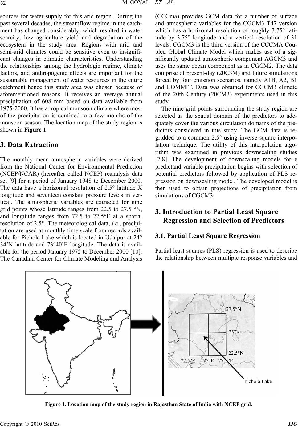

M. GOYAL ET AL.
52
sources for water supply for this arid region. During the
past several decades, the streamflow regime in the catch-
ment has changed considerably, which resulted in water
scarcity, low agriculture yield and degradation of the
ecosystem in the study area. Regions with arid and
semi-arid climates could be sensitive even to insignifi-
cant changes in climatic characteristics. Understanding
the relationships among the hydrologic regime, climate
factors, and anthropogenic effects are important for the
sustainable management of water resources in the entire
catchment hence this study area was chosen because of
aforementioned reasons. It receives an average annual
precipitation of 608 mm based on data available from
1975-2000. It has a tropical monsoon climate where most
of the precipitation is confined to a few months of the
monsoon season. The location map of the study region is
shown in Figure 1.
3. Data Extraction
The monthly mean atmospheric variables were derived
from the National Center for Environmental Prediction
(NCEP/NCAR) (hereafter called NCEP) reanalysis data
set [9] for a period of January 1948 to December 2000.
The data have a horizontal resolution of 2.5° latitude X
longitude and seventeen constant pressure levels in ver-
tical. The atmospheric variables are extracted for nine
grid points whose latitude ranges from 22.5 to 27.5 °N,
and longitude ranges from 72.5 to 77.5°E at a spatial
resolution of 2.5°. The meteorological data, i.e., precipi-
tation are used at monthly time scale from records avail-
able for Pichola Lake which is located in Udaipur at 24°
34’N latitude and 73°40’E longitude. The data is avail-
able for the period January 1975 to December 2000 [10].
The Canadian Center for Climate Modeling and Analysis
(CCCma) provides GCM data for a number of surface
and atmospheric variables for the CGCM3 T47 version
which has a horizontal resolution of roughly 3.75° lati-
tude by 3.75° longitude and a vertical resolution of 31
levels. CGCM3 is the third version of the CCCMA Cou-
pled Global Climate Model which makes use of a sig-
nificantly updated atmospheric component AGCM3 and
uses the same ocean component as in CGCM2. The data
comprise of present-day (20C3M) and future simulations
forced by four emission scenarios, namely A1B, A2, B1
and COMMIT. Data was obtained for CGCM3 climate
of the 20th Century (20CM3) experiments used in this
study.
The nine grid points surrounding the study region are
selected as the spatial domain of the predictors to ade-
quately cover the various circulation domains of the pre-
dictors considered in this study. The GCM data is re-
gridded to a common 2.5° using inverse square interpo-
lation technique. The utility of this interpolation algo-
rithm was examined in previous downscaling studies
[7,8]. The development of downscaling models for e
predictand variable precipitation begins with selection of
potential predictors followed by application of PLS re-
gression on downscaling model. The developed model is
then used to obtain projections of precipitation from
simulations of CGCM3.
3. Introduction to Partial Least Square
Regression and Selection of Predictors
3.1. Partial Least Square Regression
Partial least squares (PLS) regression is used to describe
the relationship between multiple response variables and
Figure 1. Location map of the study region in Rajasthan State of India with NCEP grid.

M. GOYAL ET AL.
53
predictors through the latent variables. PLS regression
can analyze data with strongly collinear, noisy, and nu-
merous X-variables, and also simultaneously model sev-
eral response variables, Y. In general, the PLS approach
is particularly useful when one or a set of dependent
variables (or time series) need to be predicted by a large
set of predictor variables (or time series) that are strongly
cross-correlated. This is often the case in empirical
downscaling of climate variables [11]. For details of PLS
regression, one can refer to Manne [12] and Wold [13].
3.2. Selections of Predictors
The selection of appropriate predictors is one of the most
important steps in a downscaling exercise for down-
scaling predictands. The predictors are chosen by the
following criteria: 1) predictors are skillfully predicted
by GCMs 2) they should represent important physical
processes in the context of the enhanced greenhouse ef-
fect 3) they should not be strongly correlated to each
other [14]. We have used 9 large-scale atmospheric vari-
ables, viz, air temperature (at 925,500 and 200mb pres-
sure levels), geopotential height (at 200 and 500mb
pressure levels), zonal (u) and meridional (v) wind ve-
locities (at 925 and 200mb pressure levels), as the pre-
dictors for downscaling GCM output to mean monthly
precipitation over a catchment.
The VIP (Variable Importance in the Projection)
scores obtained by the PLS regression, has been paid an
increasing attention as an importance measure of each
explanatory variable or predictor [15]. The variable se-
lection procedure under PLS is proposed with an appli-
cation to downscaling technique for identifying influ-
encing variables on understand the impact of climate
change. The VIP scores which are obtained by PLS re-
gression, can be used to select most influential variables
or predictors, X [15]. The VIP score can be estimated for
j-th X-variable by
2
1
1
(,)
(,)
k
j
diij
ki
di
i
p
VIPRY tw
RYt 



(1)
where Rd is defined as the mean of the squares of the
correlation coefficients (R) between the variables and the
component.
2
1
1
(,) (,)
k
j
i
RdX cRxc
p
 (2)
Usually the predictor variable whose VIP score is
greater than 0.8 and above is considered as an important
variable [16]. It can be seen form Figure 2 that seven
predictor variables namely air temperature at 925 mb,
500 mb and 200 mb, zonal wind (925 mb); meridoinal
wind (925 mb); zeo-potential height 500 mb and 200 mb
have their VIP score greater than 0.8. Hence, these vari-
ables are used in the prediction model to obtain projected
predictands.
Figure 2. VIP of the predictand variable (precipitation) of the three-component PLSR model.

M. GOYAL ET AL.
54
4. Downscaling of GCM Models
There are several different methods, which can be used
to derive the relationship between local and large-scale
climates. PLS regression is used to downscale mean
monthly precipitation in this study. The data of potential
predictors is first standardized. Standardization is widely
used prior to statistical downscaling to reduce bias (if
any) in the mean and the variance of GCM predictors
with respect to that of NCEP-reanalysis data [17]. Stan-
dardization is done for a baseline period of 1948 to 2000
because it is of sufficient duration to establish a reliable
climatology, yet not too long, nor too contemporary to
include a strong global change signal [8,17].
To develop downscaling models, the feature vectors
(i.e., predictors) which are prepared from NCEP record,
are partitioned into a training set and a validation set.
Feature vectors in the training set are used for calibrating
the model, and those in the validation set are used for
validation. The 26-year mean monthly observed precipi-
tation data series were broken up into a calibration period
and a validation period. The models were calibrated on
the calibration period 1975 to 1989 and validation in-
volved period 1990 to 2000. The various error criteria
are used as an index to assess the performance of the
model. Based on the latest IPCC scenario, models for
mean monthly precipitation were evaluated based on the
accuracy of the predictions for validation data set. The
following criteria of PLS regression models were chosen
in this study.
1) The Q²CUM index measures the global contribution
of the h first components to the predictive quality of the
model. The Q²CUM (h) index writes:
2
11
1
h
j
CUM jj
PRESS
QRRS


 (3)
where PRESSj PRESS being associated with a j-compo-
nent PLS model and RRSj–1 RRS being associated with a
(j-1) component PLS model. It must be as close as possi-
ble to 1.
2) The R²XCUM index is the sum of the coefficients of
determination between the explanatory variables and the
h first components. It is therefore a measure of the ex-
planatory power of the h first components for the ex-
planatory variables of the model.
22
21*100
(1)
h
ii
i
hL
tp
RX np



(4)
3) The R²YCUM index is the sum of the coefficients of
determination between the dependent variables and the h
first components. It is therefore a measure of the ex-
planatory power of the h first components for the de-
pendent variables of the model.
22
,
1)
1(1)() *100
1
L
h adjhL
n
RYRY nh






(5)
where
[]
21
2
1
ˆ
()
()
L
L
nh
ii
i
hn
ii
i
yy
RY
yy







(6)
where []h
i
y
is the prediction of the observation yi for an
h-component model and y the average of the nL observa-
tions, yi.
A comparison of proposed downscaling method with
the commonly used principal component regression was
performed. The leading principal components, which
together explain about 98% of predictor’s variability,
were retained to be used in empirical model (PCRM2)
development. The same error criteria were used to assess
the performance of model.
5. Results and Discussions
Seven predictor variables namely air temperature at 925
mb, 500 mb and 200 mb; zonal wind (925 mb); merido-
inal wind (925 mb); zeo-potential height 500 mb and 200
mb at 9 NCEP grid points with a dimensionality of 63,
are used as the standardized data of potential predictors.
These feature vectors are provided as input to the PLS
regression and PCR downscaling models. PLS regression
is performed on this dataset. Results of the PLS regres-
sion model (viz. PLSRM1) and Principal Component
based regression model (viz. PLSRM2) are tabulated in
Table 2.
Model quality indexes Q²CUM index, R²XCUM and
R²YCUM index have been shown in Table 1. It is clear that
all three indexes are highest for the three component of
for predictand precipitation. Q²CUM index, R²XCUM and
R²YCUM index are 0.647, 0.724 and 0.907, respectively.
Hence, model quality can be considered as good.
Coefficient of correlation (CC) was in the range of
0.80-0.87, RMSE was in the range of 43.20-44.98, N-S
Index was in the range of 0.58-0.75 and MAE was in the
range of 0.44-0.58 for PLS regression based model
PLSRM1 for training and validation set. For PCRM2,
Coefficient of correlation (CC) was in the range of 0.42-
0.61, RMSE was in the range of 78.18-120.45, N-S In-
dex was in the range of 0.31-0.10 and MAE was in the
range of −0.16-0.19 for PCR based model PCRM2 for
training and validation set. Hence it is clear from Table 2
that PLS regression is performed better than principal
component regression. A comparison of mean monthly
observed precipitation with precipitation simulated using
PLS regression models PLSRM1 has been shown from
Figure 3 for validation period.
Once the downscaling models have been calibrated

M. GOYAL ET AL.
55
and validated, the next step is to use these models to
downscale the control scenario simulated by the GCM.
The GCM simulations are run through the calibrated and
validated PLS regression model (viz. PLSRM1) to obtain
future simulations of predictand. The predictand (viz.
precipitation) patterns are analyzed with box plots for 20
year time slices. The middle line of the box gives the
median whereas the upper and lower edges give the 75
Table 1. Various quality measures of PLS regression model
(PLSRM1).
Precipitation (PLSRM1)
Index Comp1 Comp2 Comp3
Q²CUM 0.468 0.633 0.647
R²XCUM 0.486 0.659 0.724
R²YCUM 0.747 0.884 0.907
Figure 3. Typical results for comparison of the monthly
observed precipitation with precipitation simulated using
PLR regression downscaling model PLSRM1 for NCEP
data.
Figure 4. Box plots results from the PLS regression-based
downscaling model PLSRM1 for the predictand precipiation.
percentile and 25 percentile of the data set, respectively.
Typical results of downscaled predictand (precipitation)
obtained from the predictors are presented in Figure 4.
In part (i) of Figure 4, the precipitation downscaled us-
ing NCEP and GCM datasets are compared with the ob-
served precipitation for the study region using box plots.
The projected precipitation for 2001-2020, 2021-2040,
2041-2060, 2061-2080 and 2081-2100 for the four sce-
narios A1B, A2, B1 and COMMIT are shown in (ii), (iii),
(iv) and (v) respectively.
From the box plots of downscaled predictand (Figure
4), it can be observed that precipitation are projected to
increase in future for A1B, A2 and B1 scenarios. The
average value of observed precipitation for last 26 years
(1975-2000) is 608 millimeters. The average value of
precipitation for 100 years (2001-2100) from SRES A1B
scenario of CCCma is 677 millimeters while average

M. GOYAL ET AL.
56
Table 2. Various performance statistics of model PLSRM1 and PCRM2.
CR SSE MSE RMSE NMSE N-S Index MAE
Model Training Validation Training Validation TrainingValidation Training ValidationTrain-
ing
Valida-
tion Training Valida- tion
Train-
ing
Valida-
tion
PLSRM1 0.87 0.80 145691.44 111969.46 2023.491866.1644.9843.20 0.250.410.75 0.58 0.580.44
PCRM2 0.61 0.42 311122.00 451324.00 6112.0014509.0078.18120.450.050.030.31 0.10 −0.160.19
value of precipitation for 100 years (2001-2100) from
SRES A2 scenario of CCCma is 719 millimeters. The
mean value of precipitation for 100 years (2001-2100)
from SRES B1 scenario of CCCma is 626 millimeters
while mean value of precipitation for 100 years (2001-
2100) from COMMIT scenario of CCCma is 618 milli-
meters. Hence, it is clear that the projected increase of
precipitation is high for A1B and A2 scenarios whereas it
is least for B1 scenario.
This is because the scenario A1B and A2 have the
highest concentration of atmospheric carbon dioxide
(CO2) equal to 720 ppm and 850 ppm, while the same for
B1 and COMMIT scenarios are 550 ppm and ≈ 370
ppm respectively. Rise in concentration of atmospheric
CO2 in the atmosphere causes the earth’s average tem-
perature to increase, which in turn causes increase in
evaporation especially at lower latitudes. The evaporated
water would eventually precipitate [17]. In the COMMIT
scenario, where the emissions are held the same as in the
year 2000, no significant trend in the pattern of projected
future precipitation could be discerned. The overall re-
sults show that the projections obtained for precipitation
are indeed robust.
6. Conclusions
This paper investigates the suitability of partial least
square regression approach to downscale mean monthly
precipitation from GCM output to local scale. The effec-
tiveness of this model is demonstrated through the ap-
plication of lake catchments in arid region in India. The
predictands are downscaled from simulations of CGCM3
for four IPCC scenarios namely SRES A1B, A2, B1 and
COMMIT.
The selection of relevant predictors used for empirical
model development plays a crucial role. PLS regression
has been applied for selection of important variables
which have a VIP score greater than 0.8. PLS regression
seems to be a useful tool for downscaling. PLS regres-
sion seems to be a useful alternative to the commonly
used PCR method for empirical downscaling. The results
of downscaling models using PLS regression show that
precipitation is projected to increase in future for A2 and
A1B scenarios, whereas it is least for B1 and COMMIT
scenarios using predictors.
5. References
[1] R. Weisse and R. Oestreicher, “Reconstruction of Poten-
tial Evaporation for Water Balance Studies,” Climate Re-
search, Vol. 16, No. 2, 2001, pp. 123-131.
[2] C. Prudhomme, D. Jakob and C. Svensson, “Uncertainty
and Climate Change Impact on the Flood Regime of
Small UK Catchments,” Journal of Hydrology, Vol. 277,
No. 1, 2003, pp. 1-23.
[3] R. L. Wilby, C. W. Dawson and E. M. Barrow, “SDSM –
A Decision Support Tool for the Assessment of Climate
Change Impacts,” Environmental Modelling & Software,
Vol. 17, No. 2, 2002, pp. 147-159.
[4] M. K. Goyal and C. S. P. Ojha, “Robust Weighted Re-
gression as a Downscaling Tool in Temperature Projec-
tions,” International Journal of Global Warming. http://
www.inderscience.com/browse/index.php?journalID=331
&action=coming
[5] R. L. Wilby, “Modelling Low-Frequency Rainfall Events
Using Airflow Indices, Weather Patterns and Frontal Fre-
quencies,” Journal of Hydrology, Vol. 213, No.1-4, 1998,
pp. 380-392.
[6] A. J. Cannon and P. H. Whitfield, “Downscaling Recent
Streamflow Conditions in British Columbia, Canada Us-
ing Ensemble Neural Network Models,” Journal of Hy-
drology, Vol. 259, No. 1, 2002, pp. 136-151.
[7] S. Tripathi, V. V. Srinivas and R. S. Nanjundiah, “Down-
scaling of Precipitation for Climate Change Scenarios: A
Support Vector Machine Approach,” Journal of Hydrol-
ogy, Vol. 330, No. 3-4, 2006, pp. 621-640.
[8] S. Ghosh and P. P. Mujumdar, “Statistical Downscaling
of GCM Simulations to Streamflow Using Relevance
Vector Machine,” Advances in Water Resources, Vol. 31,
No. 1, 2008, pp. 132-146.
[9] E. Kalnay, et al., “The NCEP/NCAR 40-Year Reanalysis
Project,” Bulletin of the American Meteorological Society,
Vol. 77, No. 3, 1996, pp. 437-471.
[10] S. D. Khobragade, “Studies on Evaporation from Open
Water Surfaces in Tropical Climate,” PhD Dissertation,
Indian Institute of Technology, Roorkee, 2009.
[11] K. Bergant and L. K. Bogataj, “N-PLS Regression as
Empirical Downscaling Tool in Climate Change Studies,”
Theoretical and Applied Climatology, Vol. 81, No. 1-2,
2005, pp. 11-23.
[12] R. Manne, “Analysis of Two Partial Least Squares Algo-
rithms for Multivariate Calibration,” Chemometrics and
Intelligent Laboratory Systems, Vol. 2, No. 1, 1987, pp.
187-197.
[13] W. Svante, M. Sjostrom and L. Eriksson, “PLS-Regre-
ssion: A Basic Tool of Chemometric,” Chemometrics and
Intelligent Laboratory Systems, Vol. 58, No. 2, 2001, pp.
109-130.
[14] B. C. Hewitson and R. G. Crane, “Climate Downscaling:

M. GOYAL ET AL.
57
Techniques and Application,” Climate Research, Vol. 7,
1996, pp. 85-95.
[15] I. G. Chong and C. H. Jun, “Performance of Some Vari-
able Selection Methods When Multicollinearity is Pre-
sent,” Chemometrics and Intelligent Laboratory Systems,
Vol. 78, No. 1-2, 2005, pp. 103-112.
[16] L. Eriksson, E. Johansson, N. Kettaneh-Wold and S.
Wold, Multi- and Megavariate Data Analysis: Principles
and Applications, Umetrics Academy, Umeå, 2001.
[17] A. Anandhi, V. V. Srinivas, D. N. Kumar, R. S. Nanjun-
diah, “Role of Predictors in Downscaling Surface Tem-
perature to River Basin in India for IPCC SRES Scenar-
ios Using Support Vector Machine,” International Jour-
nal of Climatology, Vol. 29, No. 4, 2009, pp. 583-603.