Uncovering preferences from patient list data using benefit efficient models

doi:10.4236/jbise.2010.38106

Paper Menu >>

Journal Menu >>

J. Biomedical Science and Engineering, 2010, 3, 799-806 JBiSE

doi:10.4236/jbise.2010.38106 Published Online August 2010 (http://www.SciRP.org/journal/jbise/).

Published Online August 2010 in SciRes. http:// www. scirp. org/journal/jbise

Uncovering preferences from patient list data using benefit

efficient models

Jan Ubøe, Jostein Lillestøl

The Norwegian School of Economics and Business Administration, Bergen, Norway.

Email: jan.uboe@nhh.no, jostein.lillestol@nhh.no

Received 11 September 2009; revised 1 June 2010; accepted 5 June 2010.

ABSTRACT

In this paper it is shown how the benefit efficient

patient list model of Ubøe and Lillestøl [1] can be

used to infer strength of preferences from patient list

data. It is proved that the model allows the cons-

truction of unique sets of preferences replicating the

observed allocations. To illustrate how this theory can

be applied in practice, preferences are uncovered

from a small data set, obtained from the Norwegian

patient list system.

Keywords: Patient Lists; Efficient Welfare; Statistical

Distributions

1. INTRODUCTION

In the Norwegian patient list system in general practice

the patients can be assigned to a general practitio ner that

agrees to have the main responsibility for his or hers

patients. As there are limited numbers of doctors of

specific types, e.g. gender, it may happen that a signi-

ficant number of patients are assigned to doctors of the

wrong type, i.e. a type of doctor that they really do not

want. This gives rise to several interesting research

questions, among them: How can we characterize as sign -

ments that conform to reasonable criteria for total bene-

fits to the patient-doctor community, when patients are

individually competing for the scarce resource? Which

changes in allocation can be expected when the avail-

ability of the scarce resource changes, e.g. by increased

availability of female doctors? The latter is known to

happen in many countries, and was precisely the

question asked by the investigators on general practice

and community medicine that posed the problem in the

first place.

In [1] Ubøe and Lillestøl suggested a new statistical

framework for this context, enable to answer questions

of this kind, based on the concept of benefit efficiency.

The next research challenge was then to see if the model

allowed inferences, i.e., to say something about the

preference structure based on an observed allocation.

This turned out to involve some delicate theoretical

problems, among them non-uniqueness, and the purpose

of this paper is to present our solution to these problems.

As an illustration of the theory we will con sider a special

case, using patient list data from the Norwegian patient

list system in general practice. These data report the

registered allocation of male and female patients to male

and female doctors. While this is mainly a theoretical

paper, the paper also offers some guidelines for

practitioners that want to apply this kind of theory to real

world data.

The theory of this paper follows from the idea of a

benefit efficient allocation, which can be described as

follows: Let A1, A2, …, AT denote the sets of actions that

agents of type 1, 2, …, T can choose, let Ut: At R be

the real number utilities of each choice, and let Q1,

Q2, …, QT be a sequence of probability measures on A1,

A2, …, AT. Then Q = Q1 × Q2 ×…× QT is called a benefit

efficient probability measure if it satisfies the two

conditions:

 Larger aggregated utility, i.e. sum of utilities of all

agents, of an allo cation implies larger probability of that

allocation.

 As the number of agents of each type pass to

infinity, the numbers of agents making each choice must

satisfy a specified set of linear allocation constraints.

Quite surprisingly, there are extremely few probability

measures of this type. In fact when utilities and cons-

traints are given, these measures form a one parameter

family. In the inv erse problem we consider in this paper,

the parameter can be set to 1 without loss of generality.

Then the resulting allocation will be as given by For-

mula (1) in the theory section below, where we briefly

recall the model construction in [1], and then show how

we can obtain unique representations of preferences. To

enhance readability, proofs and technical arguments are

given in appendices.

The Norwegian patient list system in general practice

800 J. Ubøe et al. / J. Biomedical Science and Engineering 3 (2010) 799-806

is described in some detail in [1], and we refer to this

paper for a review of the system. Note that our modeling

framework extends beyond the Norwegian patient list

system and it can be understood without any particular

knowledge of that system. Note also that our model is

completely specified by Formula (1), and no further

knowledge of the model will be needed to understand

the issues we address in this paper.

In the application section we use our model to infer

structure and strength of preferences from observed real

world data. These data were collected from an official

panel survey of Norwegian living conditions (Levekårs-

undersøkelse n 20 0 3) .

We believe that our basic approach to this problem is

novel. It is fundamentally different from the theory of

revealed preferences in consumer theory, see e.g. [2],

and is not in any way related to the extensive economic

literature on the design of matching system in health

care, see e.g. [3]. Hence we will not enter into a

discussion of other models in this area with a different

scope.

2. METHODS

The model in [1] can be described briefly as follows:

Assume that there are S groups of patients, T types of

doctors, and let Pts denote the number of patients in

group s that has a doctor of type t, s = 1, 2, ... , S, t = 1,

2, … , T.

 Patients: We assume that there is a total of Es

patients belonging to group s, s = 1, 2, ..., S. A patient

belonging to group s is assumed to have a utility Uts of

having a doctor of type t, t = 1, 2, …, T. It may some-

times happen that a patient prefer to wait for a vacancy

of a suitable doctor rather than being assigned to a

doctor of a type that the patient dislikes. We let Pt(s+S)

denote the number of patients of type s waiting for a

doctor of type t (not being assigned to any doctor), and

let Ut(s+S) denote the utility of these patients.

 Doctors: Every doctor working within the system

is assumed to have a certain list length, i.e., a max imum

number of patients that he or she can serve. We assume

that there are Dt doctors of type t, and that these doctors

can serve a total of Lt patients, i.e., Lt is the sum of the

list lengths of all doctors of type t. Some doctors may

have vacancies, and we let Ut(2S + 1) denote the utility per

vacancy incurred by a doctor of type t.

Thus we have defined Pts and Uts for s = 1, 2, …, 2S +

1, t = 1, 2, …, T, which can then be represented by Tx(2S

+ 1) matrices P and U.

Utilities for vacancies and for being assigned to the

wrong type of doctor may of course be negative, in

which case we refer to these numbers as disutilities.

Note that the word utility is used in a broad sense as a

quantification of strength of preferences. Utilities are

hence not necessarily utilities in the von Neumann-

Morgenstern sense.

Clearly the (E1, …, ES) patients can be allocated to the

(D1, …, DT) doctors in many different ways. The basic

hypothesis in [1], however, is to assume that the system

is benefit efficient in the sense that states with large

aggregate utility (sum of the utility of all patients and

doctors) are more probable than states with smaller total

utility. If the system is benefit efficient with a large

number of patients in every group, it is possible to prove,

see [1], that the allocation will settle at a statistical

equilibrium given by the following explicit formula:

() 1,,

() 1,,2

() 21

ts ts

tsts Sts

tts

BexpUs S

D BexpUsSS

AexpUsS

















(1)

(2 1)

()

tst St

tst sSs

PP L

PP E

















See Appendix 3 on how to compute the balancing

factors A1, A2, …, AT, B1, B2, …, BS. Note that these

allocations must not be confused with the allocatio n with

maximum total utility. In fact, the allocation with maxi-

mum total utility can be obtained as special case if one

multiplies the utilities in (1) with a constant and let that

constant pass to infinity.

The basic problem we want to address in this paper

can be formulated as follows: Assume that the system is

benefit efficient and that we observe

 The total number of patients in each group, i.e. Es, s

= 1, …, S.

 The total number of doctors of each type, i.e. Dt, t

= 1, …, T.

 The total list length of doctors of each typ e, i.e. Lt, t

= 1, …, T.

 The final allocation of patients to doctors/waiting

lists, i.e. Pts, s = 1, … , 2S + 1, t = 1, … , T.

To what extent do these observations reveal the

strength of the preferences

Uts, s = 1, …, 2S + 1, t = 1, …, T ?

It is easy to observe that there are always an infinite

number of utility matrices leading to the same final

allocation. To obtain uniqueness we hence have to

impose some additional restrictions on specific utilities

and/or the relationships between them. Such restrictions

are typically based on prior knowledge of the context

and on known empirics, and modeling issu es of this kind

are discussed in detail in Section 3. In Theorem 2.1

below, we single out one of the infinitely many repre-

sentations, and refer to the representation in (2) as the

canonical choice. This is useful for two main reasons: To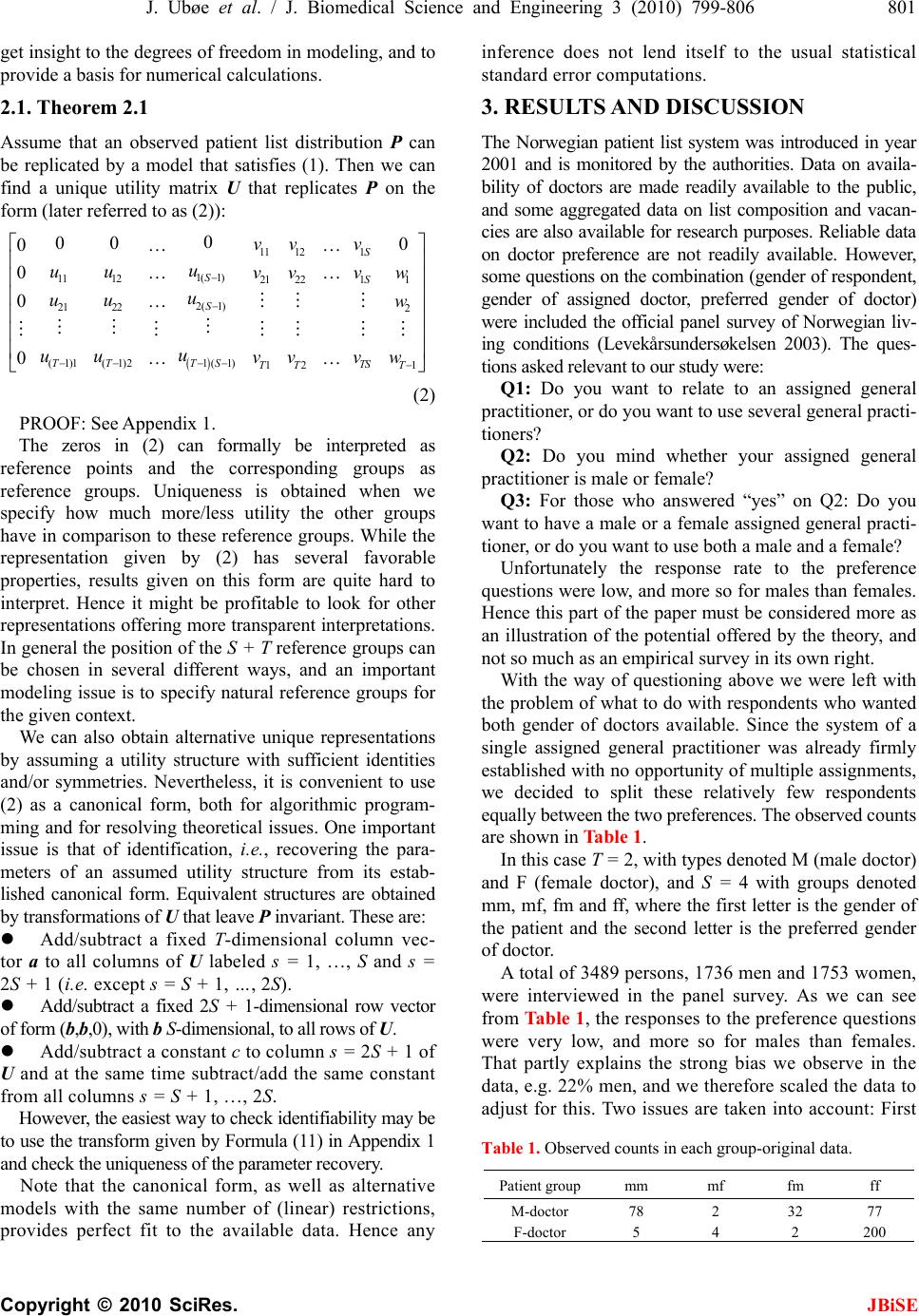

J. Ubøe et al. / J. Biomedical Science and Engineering 3 (2010) 799-806 801

get insight to the degrees of freedom in modeling, and to

provide a basis for numerical calculations.

2.1. Theor e m 2.1

Assume that an observed patient list distribution P can

be replicated by a model that satisfies (1). Then we can

find a unique utility matrix U that replicates P on the

form (later referred to as (2)):



11 12

1( 1)

11 12121 221

2( 1)

21 222

1( 1)

(1)1 (1)212 1

00 0

TT TS

TT T

uu v

vv w

uu w

uu v

vv w





 























  



(2)

PROOF: See Appendix 1.

The zeros in (2) can formally be interpreted as

reference points and the corresponding groups as

reference groups. Uniqueness is obtained when we

specify how much more/less utility the other groups

have in comparison to these reference groups. While the

representation given by (2) has several favorable

properties, results given on this form are quite hard to

interpret. Hence it might be profitable to look for other

representations offering more transparent interpretations.

In general the position of the S + T reference groups can

be chosen in several different ways, and an important

modeling issue is to specify natural reference groups for

the given context.

We can also obtain alternative unique representations

by assuming a utility structure with sufficient identities

and/or symmetries. Nevertheless, it is convenient to use

(2) as a canonical form, both for algorithmic program-

ming and for resolving theoretical issues. One important

issue is that of identification, i.e., recovering the para-

meters of an assumed utility structure from its estab-

lished canonical form. Equivalent structures are obtained

by transformations of U that leave P invariant. These are:

 Add/subtract a fixed T-dimensional column vec-

tor a to all columns of U labeled s = 1, …, S and s =

2S + 1 (i.e. except s = S + 1, …, 2S).

 Add/subtract a fixed 2S + 1-dimensional row vector

of form (b,b,0 ), with b S-dim ensional , to all rows of U.

 Add/subtract a constant c to column s = 2S + 1 of

U and at the same time subtract/add the same constant

from all columns s = S + 1, …, 2S.

However, the easiest way to check identifiab ility may be

to use the transform given by Formula (11) in Appendix 1

and check the uniqueness of the parameter recovery.

Note that the canonical form, as well as alternative

models with the same number of (linear) restrictions,

provides perfect fit to the available data. Hence any

inference does not lend itself to the usual statistical

standard error computations.

3. RESULTS AND DISCUSSION

The Norwegian patient list system was introduced in year

2001 and is monitored by the authorities. Data on availa-

bility of doctors are made readily available to the public,

and some aggregated data on list composition and vacan-

cies are also av ailable for research purposes. Reliable data

on doctor preference are not readily available. However,

some questions on the combination (gender of respondent,

gender of assigned doctor, preferred gender of doctor)

were included the official panel survey of Norwegian liv-

ing conditions (Levekårsundersøkelsen 2003). The ques-

tions asked relevant to our study were:

Q1: Do you want to relate to an assigned general

practitioner, or do you want to use several general practi-

tioners?

Q2: Do you mind whether your assigned general

practitioner is male or female?

Q3: For those who answered “yes” on Q2: Do you

want to have a male or a female assigned general practi-

tioner, or do you want to use both a male and a female?

Unfortunately the response rate to the preference

questions were low, and more so for males than females.

Hence this part of the paper must be considered more as

an illustration of the potential offered by the theory, and

not so much as an empirical survey in its own right.

With the way of questioning above we were left with

the problem of what to do with respondents who wanted

both gender of doctors available. Since the system of a

single assigned general practitioner was already firmly

established with no opportun ity of multiple assignments,

we decided to split these relatively few respondents

equally between the two preferences. The observed counts

are shown in Table 1.

In this case T = 2, with types denoted M (male doctor)

and F (female doctor), and S = 4 with groups denoted

mm, mf, fm and ff, where the first letter is the gender of

the patient and the second letter is the preferred gender

of doctor.

A total of 3489 persons, 1736 men and 1753 women,

were interviewed in the panel survey. As we can see

from Table 1, the responses to the preference questions

were very low, and more so for males than females.

That partly explains the strong bias we observe in the

data, e.g. 22% men, and we therefore scaled the data to

adjust for this. Two issues are taken into account: First

Table 1. Observed counts in each group-original data.

Patient group mm mf fm ff

M-docto

782 32 77

F-docto

54 2 200

802 J. Ubøe et al. / J. Biomedical Science and Engineering 3 (2010) 799-806

we have scaled the data so that there is an equal num-

ber of respondents of each sex, second we have scaled

the data to get the marginal frequencies in accordance

with the approximately known distribution of doctors at

the time, namely 70% male doctors and 30% female

doctors.

The results after these scalings are given in Tab le 2

per 1000 respondents.

3.1. Missing Data and Partial Information

Officially there are no waiting lists, and data on this are

hard to get. In Appendix 2, however, we prove that one

can infer the correct preferences for the groups in Table

2 even in the case where data on waiting lists and

vacancies are missing. The crucial result, Theorem 5.4,

states that these preferences are independent of the data

for waiting lists and vacancies.

A survey made by the Norwegian Ministry of Health

and Care Services (2004) r eports a total of 2 026 doctors

with vacancies, the average number of vacancies being

223. With the reported 4 563 751 patients served, this

gives 99 vacancies per 1 000 patients. For illustrative

purposes we round this in Table 3 to 100 patients per

1000 served. We have no information on how this is

distributed among the gender of doctors. If they are

distributed evenly among the genders, the number will

be as given in the parentheses in Ta ble 3 . Note that the

number of patients who want a doctor of the same

gender is higher for males than for females.

3.2. Inferring Canonical Utilities from

Observed Data

The utility matrix corresponding to the types and

groups in Table 3 is

1518 191114

2528 29

21 24

UUU











U (3)

where the row order is M, F and the column order is

mm, mf, fm, ff, mm-w, mf-w, fm-w, ff-w, vacancy,

where w indicates a waiting list state. According to

Theorem 5.4 in Appendix 2, the missing data in Table

3 can be chosen arbitrarily. Zero entries can be handled,

but unless special care is taken such entries lead to

serious numerical problems. For simplicity we have

carried out all the calculations using the numbers

reported in Table 4. We remark, however, that the

numbers reported on waiting lists are fictitious but to

some extent realistic.

To find replicating utilities, we use the construction

described in Proposition 5.3 in Appendix 1. The result is

shown in Table 5.

The numbers in parenthesis are based on the fictitious

waiting list numbers. Hence the strength of preferences

we can infer from the data in Table 2 is given by Table 6.

If we take the canonical structure as our model, we

may infer that that the patients with preference for the

scarce gender (female doctors), have high utilities for

correct matching compared with the reference groups,

and that female patients wanting a male doctor while

being assigned to a female doctor tend to have utilities

slightly below the reference group zero.

Be aware, however, that this inference may be due to

technical artifacts linked to the implicit assumptions

caused by a special choice of reference groups. The

canonical choice corresponds to an assumption where

male patients wanting a male doctor are in effect

indifferent to the gender of their doctor, and that may

very well be an artificial assumption.

3.3. Modeling and Further Inference

We will now look into the modeling aspects of alter-

native representations. While the utilities reported in

Table 5 are the unique utilities on the form (2) that

replicates the counts in Ta ble 4, there are several other

utility matrices that offer perfect replication. Also,

observations of this type are subject to considerable

amounts of randomness. Perfect replication is hence

relatively unimportant, and models offering less than

perfect fit may be superior if they carry more transparent

information.

A main issue in this context is to quantify disutilities

of incorrect patient/doctor matching. It is straight-

forward to verify that the solution of (1) is fixed if we

add the same constant to all utilities within the same

group, i.e., our model is sensitive to utility differences

but does not depend on the general level of utility.

Without loss of generality we can hence assume that all

utilities for correct patient/doctor matching are equal to

zero. These assumptions lead us to consider utility

matrices on the form:

21314141112

1323 24 2

21 22

abbc

ab b

aa bbc















U (4)

Table 2. Adjusted data from Table 1.

Patient group mm mf fm ff

M-doctor 455 12 69 164

F-doctor 19 14 2 265

Total 474 26 71 429

Table 3. Scaled counts in each group per 1000 patients served.

Patient groupmm mffmffmm-w mf-w fm-wff-wvac

M-doctor 4551269164 - - - -(70)

F-doctor 19142265 - - - -(30)

Total 4742671429 - - - -100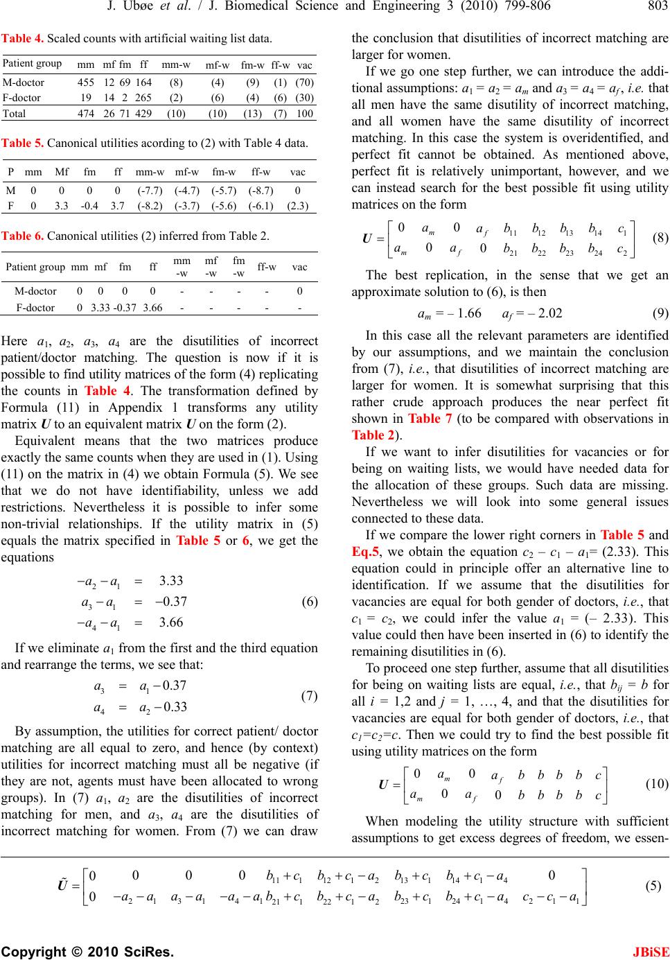

J. Ubøe et al. / J. Biomedical Science and Engineering 3 (2010) 799-806 803

Table 4. Scaled counts with artificial waiting list data.

Patient group mm mf fm ff mm-w mf-w fm-wff-wvac

M-doctor 455 12 69 164 (8) (4) (9) (1)(70)

F-doctor 19 14 2 265 (2) (6) (4) (6)(30)

Total 474 26 71 429 (10) (10) (13) (7)100

Table 5. Canonical utilities acording to (2) with Table 4 data.

P mm Mf fm ff mm-wmf-w fm-w ff-wvac

M 0 0 0 0 (-7.7) (-4.7) (-5.7) (-8.7)0

F 0 3.3 -0.4 3.7 (-8.2) (-3.7) (-5.6) (-6.1)(2.3)

Table 6. Canonical utilities (2) inferred from Table 2.

Patient group mm mf fm ff mm

-w mf

-w fm

-w ff-w vac

M-doctor 0 0 0 0 - - - - 0

F-doctor 0 3.33 -0.37 3.66 - - - - -

Here a1, a2, a

3, a

4 are the disutilities of incorrect

patient/doctor matching. The question is now if it is

possible to find utility matrices of the form (4) rep lic at in g

the counts in Table 4. The transformation defined by

Formula (11) in Appendix 1 transforms any utility

matrix U to an equivalent matrix U on the form (2).

Equivalent means that the two matrices produce

exactly the same counts when they are used in (1). Using

(11) on the matrix in (4) we obtain Formula (5). We see

that we do not have identifiability, unless we add

restrictions. Nevertheless it is possible to infer some

non-trivial relationships. If the utility matrix in (5)

equals the matrix specified in Ta b le 5 or 6, we get the

equations

3.33

0.37

3.66

 



 

(6)

If we eliminate a1 from the first and the third equation

and rearrange the terms, we see that:

0.37

0.33



 (7)

By assumption, the utilities for correct patient/ doctor

matching are all equal to zero, and hence (by context)

utilities for incorrect matching must all be negative (if

they are not, agents must have been allocated to wrong

groups). In (7) a1, a

2 are the disutilities of incorrect

matching for men, and a3, a

4 are the disutilities of

incorrect matching for women. From (7) we can draw

the conclusion that disutilities of incorrect matching are

larger for women.

If we go one step further, we can introduce the addi-

tional assumptions: a1 = a2 = am and a3 = a4 = af , i.e. th at

all men have the same disutility of incorrect matching,

and all women have the same disutility of incorrect

matching. In this case the system is overidentified, and

perfect fit cannot be obtained. As mentioned above,

perfect fit is relatively unimportant, however, and we

can instead search for the best possible fit using utility

matrices on the form

13 14111 12

23 24 2

21 22

abbc

abb

aa bbcbb















U (8)

The best replication, in the sense that we get an

approximate solution to (6), is then

am = – 1.66 a

f = – 2.02 (9)

In this case all the relevant parameters are identified

by our assumptions, and we maintain the conclusion

from (7), i.e., that disutilities of incorrect matching are

larger for women. It is somewhat surprising that this

rather crude approach produces the near perfect fit

shown in Ta b l e 7 (to be compared with observations in

Table 2).

If we want to infer disutilities for vacancies or for

being on waiting lists, we would have needed data for

the allocation of these groups. Such data are missing.

Nevertheless we will look into some general issues

connected to these data.

If we compare the lower right corners in Ta ble 5 and

Eq.5, we obtain the equation c2 – c1 – a1= (2.33). This

equation could in principle offer an alternative line to

identification. If we assume that the disutilities for

vacancies are equal for both gender of doctors, i.e., that

c1 = c2, we could infer the value a1 = (– 2.33). This

value could then have been inserted in (6) to identify the

remaining disutilities in (6).

To proceed one step fu rther, assume that all disutilities

for being on waiting lists are equal, i.e., that bij = b for

all i = 1,2 and j = 1, …, 4, and that the disutilities for

vacancies are equal for both gender of doctors, i.e., that

c1=c2=c. Then we could try to find the best possible fit

using utility matrices on the form

aabbbbc















U (10)

When modeling the utility structure with sufficient

assumptions to get excess degrees of freedom, we essen-

131 14 1411112 12

2131 412312414211

21 12212

000 0

bcbca

bcb ca

aaaaaab cb cacca

bcbca



 

 

 



 



U (5)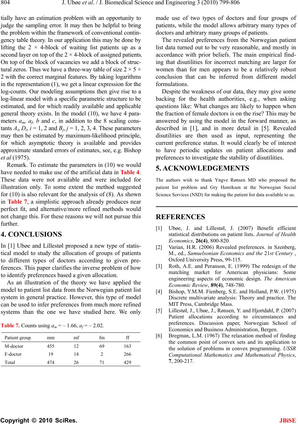

804 J. Ubøe et al. / J. Biomedical Science and Engineering 3 (2010) 799-806

tially have an estimation problem with an opportunity to

judge the sampling error. It may then be helpful to bring

the problem within the framework of conventional contin-

gency table theory. In our application this may be done by

lifting the 2 × 4-block of waiting list patients up as a

second layer on top of the 2 × 4-block of assigned patients.

On top of the block of vacancies we add a block of struc-

tural zeros. Thus we have a three-way table of size 2 × 5 ×

2 with the correct marginal features. By taking logarithms

in the representation (1), we get a linear expression for the

log-counts. Our modeling assumptions then give rise to a

log-linear mod el with a specific p arametric st ructure to be

estimated, and for which readily available and applicable

general theory exists. In the model (10), we have 4 para-

meters am, af, b and c, in addition to the 8 scaling cons-

tants Ai, Di, i = 1, 2 and Bj, j = 1, 2, 3, 4. These parameters

may then be estimated by maximum-likelihood principle,

for which asymptotic theory is available and provides

approximate standard errors of estimates, see, e.g. Bishop

et al (1975).

Remark. To estimate the parameters in (10 ) we would

have needed to make use of the artificial data in Table 4.

These data were not available and were included for

illustration only. To some extent the method suggested

for (10) is also relevant for the analysis of (8). As shown

in Ta b l e 7 , a simplistic approach already produces near

perfect fit, and alternative/more refined methods would

not change this. For these reasons we will not pursue this

further.

4. CONCLUSIONS

In [1] Ubøe and Lillestøl proposed a new type of statis-

tical model to study the allocation of groups of patients

to different types of doctors according to given pre-

ferences. This paper clarifies the inverse problem of how

to identify preferences based a given allocation.

As an illustration of the theory we have applied the

model to patient list data from the Norwegian patient list

system in general practice. However, this type of model

can be used to infer preferences from much more refined

systems than the one we have studied here. We only

Table 7. Counts using am = – 1.66, af = – 2.02.

Patient group mm mf fm ff

M-doctor 455 12 69 163

F-doctor 19 14 2 266

Total 474 26 71 429

made use of two types of doctors and four groups of

patients, while the mod el allows arbitrary many types of

doctors and arbitrary many groups of patients.

The revealed preferences from the Norwegian patient

list data turned out to be very reasonable, and mostly in

accordance with prior beliefs. The main empirical find-

ing that disutilities for incorrect matching are larger for

women than for men appears to be a relatively robust

conclusion that can be inferred from different model

formulations.

Despite the weakness of our data, they may give some

backing for the health authorities, e.g., when asking

questions like: What changes are likely to happen when

the fraction of female doctors is on the rise? This may be

answered by using the model in the forward manner, as

described in [1], and in more detail in [5]. Revealed

disutilities are then used as input, representing the

current preference status. It would clearly be of interest

to have periodic updates on patient allocations and

preferences to investigate the stability of disu tilities.

5. ACKNOWLEDGEMENTS

The authors wish to thank Yngve Rønsen MD who proposed the

patient list problem and Gry Henriksen at the Norwegian Social

Science Services (NSD) for making the patient list data available to us.

REFERENCES

[1] Ubøe, J. and Lillestøl, J. (2007) Benefit efficient

statistical distributions on patient lists. Journal of Health

Economics, 26(4), 800-820.

[2] Varian, H.R. (2006) Revealed preferences. in Szenberg,

M., ed., Samuelsonian Economics and the 21st Century ,

Oxford University Press, 99-115.

[3] Roth, A.E. and Peranson, E. (1999) The redesign of the

matching market for American physicians: Some

engineering aspects of economic design. The American

Economic Review, 89(4), 748-780.

[4] Bishop, Y.M.M. Fienberg, S.E. and Holland, P.W. (1975)

Discrete multivariate analysis: Theory and practice. The

MIT Press, Cambridge Mass.

[5] Lillestøl, J., Ubøe, J., Rønsen, Y. and Hjortdahl, P. (2007)

Patient allocations according to circumstances and

preferences. Discussion paper, Norwegian School of

Economics and Business Administration, Bergen.

[6] Bregman, L.M. (1967) The relaxation method of finding

the common point of convex sets and its application to

the solution of problems in convex programming. USSR

Computational Mathematics and Mathematical Physics,

7, 200-217.

J. Ubøe et al. / J. Biomedical Science and Engineering 3 (2010) 799-806 805

APPENDICES

Appendix 1: Proof of Theorem 2.1

Consider the following matrix transformation

11 11

1()1(21)

11(21)11

1, ,

1,, 2

ts ts

tstss SS

ts tS

UUUUs S

UUU UsSS

UUUUsS





 



 



 



 (11)

LEMMA 5.1

Let



UUbe given, let {}

UU



be defined by

(11) and let

and

 denote the corresponding

distributions of patients in (1) when we use U and U

,

respectively. Then

P.

PROOF

Let A1, …, AT, B1, …, BS denote the balancing factors

solving (1) when we use U, and define



111

12 1

112 1

exp1, ,

exp1,,

ttt

sss

AUA

UUtT

BUUsS









 (12)

If s = 1, …, S we get

exp( )exp( )

t stst sts

ABUAU B

 (13)

If s = S + 1, …, 2S we get

 



 

1121

exp( )exp

exp( )

tsStstsSsS S

ts sS S

tsSts

DDBUU

UU U















(14)

If s = 2S + 1 we get



111

12 1

111

12 1

exp( )exp()

exp( )

ttstt S

ts tS

tts

AUU U

UUU











(15)

which proves the lemma.

PROPOSIT ION 5.2

Let (1)

U and (2)

U denote two utility matrices, and

assume that (1) (2)



P in (1). Using the transforma-

tion in (11) we have (1) (2)

UU



PROOF

We have to prove that the balancing factors must be

equal, and then it follows from (1) that all the utilities

must be equal as well. It follows from Lemma 2.1 that

(1) (2)





P, and observe from (11) that (1)

1(2 1)S

U





(2)

1(2 1)0

U

 b y definition. Since

(1)(1)(2)(2)

11(21)11(2 1)

exp( )exp( )

AU AU







(16)

it follows that (1) (2)

AA



. Now put t = 1 and s = 1, …,

S, and observe from (11) that (1) (2)

UU

 by

definition. Hence from (1) we get

(1)(1) (1)(2)(2) (2)

1s11s1

exp( )exp()

AB UABU



 

(17)

Since (1) (2)

AA



it follows that (1) (2)

B



for all s

= 1, …, S. We then put s = 1 and t = 1, …, T, and

observe from (11) that (1) (2)

UU

 by definition.

From (1) again we get

(1)(1) (1)(2)(2) (2)

111 1

exp( )exp()

tttt

AB UBUA



 (18)

Since (1) (2)

B



it follows that (1) (2)

AA



for all

t = 1, …, T. We have hence proved the proposition.

Proof of Theorem 2.1

By assumption we can find a matrix U that replicates

According to Lemma 5.1 U

 also replicates

. By

construction U

 is on the special format given by (2).

Hence there exists a matrix on the form (2) that

replicates

. Conversely if a matrix is of the form

given by (2), it does not change when we apply the

transformation given by (11). Uniqueness then follows

from Proposition 5.2.

PROPOSIT ION 5.3

Let{}

obs

P be the observed numbers on the patient lists.

The replicating matrix in Theorem 2.1 can then be

constructed as follows. Put:

ln()1, ,

ln(/)1, ,2

ln()2 1

obs

tsts t

obs

PifsS

UPDifsSS

PifsS













(19)

If we put 1



, 1



in (1), it is easy to verify that

the model in (1) replicates the observed pattern. The

unique replicating matrix in Theorem 2.1 can then be

found applying the transformation in (11) to the utilities

in (19).

Appendix 2: Inference under Partial

Information

Assume that we know the number of patients on the

patient lists and the number of vacancies, but do not

know how many patients that are waiting for a vacancy.

Is it then possible to infer the strength of preferences of

the patients on the patient lists? The answer is yes, and

this can be demonstrated as follows:

Assume that(0)

P s = 1, …, S, t = 1, …, T is given,

and let (1)

P and (2)

P be arbitrary numbers for s = S +

1, …, 2S + 1, t = 1, …, T. Define the following aggre-

gated quantities

806 J. Ubøe et al. / J. Biomedical Science and Engineering 3 (2010) 799-806

(0)(0) (0)(0)

ttst ts

LPE P





()() ()()

,,1,2

iiii

ttssts

SS T

LPEPi



 





THEOREM 5.4

For i = 1,2 put (0)( )(0)( )

ttts ss

LLEEE and find a

unique matrix ()i

U of the form (2) such that the system

given by (1) replicates the numbers

(0)

()

1,, ,1,,

1,, 21

ts i

PifsSt T

PPifsS S

 







 



 (20)

If (2) (1)

1(2 1)1(2 1)

KP P



 then the two utility matrices

(1)

Uand (2)

Uare connected through the formula (here

referred to as Eq.21):



(1)

(2)(1)

(1)

1, ,,1,,

lnln()1, ,2,1, ,

lnln( )21,1,,

ts ts

UsStT

UUKsSSt T

UKsStT





 





 









 









PROOF

Define a new utility matrix 

U by the right hand side of

(21) and let (1)

A, t = 1, …, T and (1 )

s = 1, …, S

denote the balancing factors solving (1) using the

replicating utilities (1)

U Now put (2) (1)

AAK

and

(2)

B(1) /

If s = 1, …, S, t = 1, …, T w e get by (1)

 

 

(2) (2)(1)

111 (0)

exp( )/()

exp( )

ts tst sts

t ststs

ABAKBKexp U

AB U







If s = S + 1, …, 2S, t = 1, … , T we get by (1)





(2)

(1) (2)

(1)

exp( )

/(lnln( ))

ln()

tsSts

ts ts

DB KexpUK

PPK















If s = 2S + 1, t = 1, …, T we get by (1)

 



(2) (1)

exp()(lnln( ))

ttst ts

UAKexp UK











(2)

(1) (2)

(1)

ts ts

 

The marginal con strain ts are au tomatically sa tisfied when

the model re plicates each ent ry in the matrix. Note that



12 1

(1) (1)

1(21)11

12 1

lnln0

Ss ts

UU KU

















and that if s = 1, …, S , then ts ts

UU

. This proves that



Uis of the form (2). Hence if we put (2)





UU this

matrix is the unique matrix on the form (2) that

replicates the system in (20) when i = 2.

As we can see from Theorem 6.1, the utilities s

= 1, …, S, t = 1, …, T do not depend on the values of

P for s = S + 1, …, 2S + 1, t = 1, …, T. Hence we

have the following corollary:

COROLLARY

Assume that ts

P s = 1, …, S, t = 1,…,T are known,

while data on ts

P for s = S + 1, …, 2S + 1, t = 1, …, T

are missing. If we choose 0

P for s = S + 1,…, 2S

+ 1, t = 1,…,T arbitrarily, we can still infer the correct

values on ts

Ufor s = 1, …, S, t = 1, …, T.

Remark. From the bottom line in Formula (21) we see

that we can also obtain strength of preferences for

vacancies in cases where information on the number of

patients waiting for vacancies is missing. Clearly,

however, it is impossible to infer strength of preferences

for groups of patients waiting for vacancies unless we

have data for these groups.

Appendix 3: Numerical Methods

How to find a numerical solution to (1) when utilities U

and marginal constraints L and E are given? We need to

find numerical values for the S + T balancing factors

A1, …, AT, B1, …, BS. This is done as follows:

Initially we put all the balancing factors equal to 1.

Then for t = 1, …, T we update At using



(2 1)

1exp

ststS

ABUP







 (22)

Once these are updated, then for s=1,…,S we update

Bs using



()

1(expexp)

ttsttsS

BAUDU







 (23)

We then repeat the updates in (22) and (23) until the

system settles. The algorithm is a variant of the Bregman

balancing algorithm, see Bregman (1967). Like the stan-

dard Bregman algorithm this algorithm is surprisingly

efficient, and solves large systems in a very short time.