J. Biomedical Science and Engineering, 2010, 3, 791-798 JBiSE
doi:10.4236/jbise.2010.38105 Published Online August 2010 (http://www.SciRP.org/journal/jbise/).
Published Online August 2010 in SciRes. http:// www. scirp. org/journal/jbise
Innovative data mining approaches for outcome prediction of
trauma patients
Eleni-Maria Th eodorak i1, Stylianos Katsaragakis2, Christos Koukouvinos3, Chr i st i n a Par p ou l a 3
1Department of Statistics and Actuarial-Financial Mathematics, University of the Aegean, Samos Island, Greece;
2First Propaedeutic Surgery Clinic, Hippocratio Hospital, Athens, Greece;
3Department of Mathematics, National Technical University of Athens, Athens, Greece.
Received 7 June 2010; revised 17 June 2010; accepted 23 June 2010.
ABSTRACT
Trauma is the most common cause of death to young
people and many of these deaths are preventable [1].
The prediction of trauma patients outcome was a
difficult problem to investigate till present times. In
this study, prediction models are built and their ca-
pabilities to accurately predict the mortality are as-
sessed. The analysis includes a comparison of data
mining techniques using classification, clustering and
association algorithms. Data were collected by Hel-
lenic Trauma and Emergency Surgery Society from
30 Greek hospitals. Dataset contains records of 8544
patients suffering from severe injuries collected from
the year 2005 to 2006. Factors include patients' de-
mographic elements and several other variables reg-
istered from the time and place of accident until the
hospital treatment and final outcome. Using this
analysis the obtained results are compared in terms
of sensitivity, specificity, positive predictive value and
negative predictive value and the ROC curve depicts
these methods performance.
Keywords: Data Mining; Medical Data; Decision Trees;
Classification Rules; Association Rules; Clusters;
Confusion Matrix; ROC
1. INTRODUCTION
One of the most common and rapidly growing causes
of death and disability worldwide, regardless of each
country’s development level, is traumatic injury [2].
Every day 16,000 people die [3] and trauma is the
leading cause of death in the age of 44 years [4] and the
fourth leading cause of all ages after cardiovascular,
neoplastic, and respiratory diseases. In 1996 the Na-
tional Academy of Sciences and National Research
Council published a report which characterized the
injury as the “neg lec ted disea se of the modern world”.
Due to technological advancements in healthcare
domain, an enormous amount of data has been col-
lected over the last few years. This fact is followed by
clinician’s willingness to explore different technologies
and methodologies to analyze these data because their
assessment may lead to trends and patterns within the
data previously unknown which could significantly
enhance their understanding of disease management.
Interest in developing prognostic models for binary
outcomes has emerged as an essential tool for evalua-
tion of medical treatment. Multiple models exist to as-
sist with prediction of the outcome of injured patients
and many comp arisons be tween different methods exist
[4]. Traditionally, researchers have used the regression
techniques which are not ideal in handling multidimen-
sional, complex biologic data stored in large databases
and are time consuming. Therefore, due to the fact that
there is no consensus as to an optimal method, it is in-
teresting to explore different methods.
Data mining methods were developed to overcome
these limitations. With these techniques, a priori know-
ledge of variable associations is unnecessary. In con-
trast to an a priori approach to the selection of predictor
variables, data mining allows the discovery of previ-
ously unknown variable relationships by exploring a
wide range of possible predictor variables. The process
of data mining is to find hidden patterns and associa-
tions in the data. The utility of data mining methods to
derive medical prognostic models from retrospective
data, can contribute to increased availability and vol-
ume of medical data gathered through systematic use of
laboratory, clinical and hospital information systems.
Also, it can lead to construction of interpretable prog-
nostic models, handling of noise and missing values,
and discovery and incorporation of non-linear patterns
and feature combinations.
This paper investigates the utility of machine learn-
ing techniques to construct outcome prediction models

792 E.-M. Theodoraki et al. / J. Biomedical Science and Engineering 3 (2010) 791-798
for severe trauma patients and examines measures that
will improve the quality of treatment and therefore sur-
vivability of patient through optimal management. The
study is organized as follows. Section 2 introduces the
dataset that was used to investigate the plausibility of
modeling the outcome. Statistical methods used for that
purpose were classification, association and clustering
algorithms. The results of data analysis, and their eval-
uation according to their predictive ability are reported
in Section 3. Section 4 summarizes the results and pro-
vides conclusion of the paper.
2. MATERIALS AND METHODS
2.1. Patient Population and Variables
Our database consisted of cases collected during the
project, entitled “Report of the epidemiology and man-
agement of trauma in Greece”, which was initiated in
October 2005 and lasted for twelve months. Study in-
cluded patients from a range of 30 teaching, and general
hospitals who were admitted w ith a primary diagnosis of
injury. Information was gathered for these trauma pa-
tients admitted for at least one day in hospital. To avoid
biasing estimates, persons who arrived dead or died at
the Emergency Room of each hospital were excluded
from the analysis. The data and injury scoring was per-
formed by a highly-trained coordinator.
Input variables which were extracted and included to
the models concerned demographics, mechanism of in-
jury, month of admission to hospital, whether the patient
was referred from another hospital, prehospital care,
hospital care and procedures, and outcomes at discharge.
Various injury severity scores were also considered in-
cluding Injury Severity Score (ISS) [5], Abbreviated
Injury Scores (AIS) [6], and the Glasgow Coma Score
(GCS) [7]. For all models, there was a single output
variable: probability of death.
Trauma registry was followed by extensive correction
and verification of the data. During preprocessing an aly-
sis missing data were also handled. Despite the chal-
lenges inherent when data are missing, information
could be gained when a thoughtful and systematic ana-
lytical approach is used [8]. For that purpose Multiple
imputation (MI) was an appropriate method that was
used to handle Missing At Random Data in our dataset
[9] in order to minimize bias and increase the validity of
findings. In this method, multiple (m) versions (typical
range 5-20) of the data set are created using available
data to predict missing values. These data sets are then
used to conduct m analyses, which are then combined
into one inferential analysis. The particular appeal of this
method is that once completed data sets have been de-
veloped, standard statistical methods can be used. Ad-
justing multiple imputation issues to data mining meth-
ods, derived datasets were compared in terms of per-
formance (correctly classified datasets) and the one with
the most correctly classified training and test sets was
chosen.
The analysis was carried out using the SPSS 17.0 and
SPSS Clementine 12.0 statistical software.
2.2. Data Mining Algorithms
In this section, we present the data mining methods that
were applied to analyze the trauma data. These methods
may be categorized according to their goal as feature
selection methods, decision tree learners, binary classi-
fier comparison metrics, clustering algorithms and gen-
eralized rule induction algorithms.
2.2.1. F eature S e lection
In order to reduce data set size, minimize the computa-
tional time and improve model accuracy, a set of vari-
ables selection criteria may be used. Such criteria are the
maximum percentage of records in a single category
criterion, as fields which have too many records falling
into the same category may be omitted and the maxi-
mum number of categories as a percentage of records
criterion, as if a high percentage of the categories con-
tains only a single case, the field may be ignored. There
are two more variable selection criteria, the minimum
standard deviation criterion and the minimum coefficient
of variation criterion. According to these, fields with
standard deviation or respectively coefficient of variance
less than or equal to the specified minimum measure
may be of limited use. The coefficient of variance is de-
fined as the ratio of the predictor standard deviation to
the predictor mean.
A common technique used in data mining is ranking
the attributes based on the measure of importance which
is defined as (1-p), where p is the p-value of a chosen
statistical test such as the Pearson's chi-square statistic,
the Likelihood-ratio chi-square statistic, the Cramer’s V
or Lambda statistic. More details can be found among
others in [10-12] and [13]. The Pearson’s chi-square sta-
tistical test, is a test of independence between X, where
X is a predictor with I categories, and Y, where Y is the
target value with J categories, that involves the differ-
ence between the observed and the expected frequencies.
The expected cell frequencies under the null hypothesis
of independence are estimated by ..
ˆij
ij
NN
NN , where
N is the total number of cases, ij
N is the number of
cases with X = i and Y = j, .i N is the number of cases
with X = i (.1
J
iij
j
NN



) and .
j
N is the number of cases
with Y = j (.1
I
j
ij
i
NN



).

E.-M. Theodoraki et al. / J. Biomedical Science and Engineering 3 (2010) 791-798 793
Under the null hypothesis, Pearson’s chi-square con-
verges asymptotically to a chi-square distribution 2
d
x
with degrees of freedom d = (I – 1)(J – 1). Now, the
p-value based on Pearson’s chi-square 2
X
is calculated
by p-value = Prob 22 ()
d
x
X, where
22
11
ˆˆ
()/
IJ
ij ijij
ij
X
NN N


 .
2.2.2. De c ision Trees
Decision tree models are a structural description which
gives the opportunity to develop classification models
that may be used to predict or classify future data sets,
according to a number of provided decision rules. Future
data with unknown classification may be classified just
by routing down the tree according to the tests in nodes
and assigning the class of the reached leaf. Some of the
advantages of this approach are that it is easy under-
standable, can be transformed into a set of rules (if-then
rules) that interpret the data set and finally that the pro-
vided tree includes only the important attributes that
really contribute to the decisions making. The Classifi-
cation and Regression Tree (C&RT) is a method based
on recursive partitioning to split the training set into
subsets so as to obtain more homogeneous subsets than
in the previous step. The split is based on the reduction
in an impurity index, and in this study we used the Gini
index. CHAID algorithm, or Chi-square Automatic In-
teraction Detection, is based on the significance level of
a statistical test and is a non-binary tree method, that is,
it can produce more than two categories at any particular
level in the tree. C5.0 algorithm works for data sets
where the target field is categorical and builds decision
tree by splitting the sample based on the field that pro-
vides the maximum information gain at each level.
2.2.3. Clustering
Clustering is concerned with grouping records with re-
spect to similarity of values for a set of input fields
without the profit of prior knowledge about the form and
the characteristics of the groups.
K-means is an iterative algorithm which tries to dis-
cover k clusters, where (k) is defined by the user, so that
records within a cluster are similar to each other and
distinct from records in other clusters. There are differ-
ent distance measures, such as Euclidean distance,
Manhattan distance and Mahalanobis distance, but in our
application we used the Euclidean distance.
The TwoStep cluster method is a scalable cluster
analysis algorithm designed to handle very large data
sets and both continuous and categorical variables or
attributes. It requires only one data pass. It has two steps
1) pre-cluster the cases (or records) into many small
sub-clusters 2) cluster the sub-clusters resulting from
pre-cluster step into the desired number of clusters. The
TwoStep algorithm uses an hierarchical clustering me-
thod in the second step to assess multiple cluster solu-
tions and automatical ly determine the o ptimal nu mber of
clusters for the input data. To determine the number of
clusters automatically, TwoStep uses a two-stage proce-
dure that works well with the hierarchical clustering
method. In the first stage, the BIC (distance measure) for
each number of clusters within a specified range is cal-
culated and used to find the initial estimate for the num-
ber of clusters. TwoStep can use the hierarchical cluster-
ing method in the second step to assess multiple cluster
solutions and automatically determine the optimal num-
ber of clusters for the input data.
2.2.4. Association Rules
Association rule mining finds interesting associations
and/or correlation relationships among large set of data
items. Association rules show attribute value conditions
that occur frequently together in a given data set. A typ-
ical and widely-used example of association rule mining
is Market Basket Analysis. Association rules provide
information of this type in the form of if-then statements.
These rules are computed from the data and, unlike the
if-then rules of logic, association rules are probabilistic
in nature. In association analysis the antecedent and
consequent are sets of items (called itemsets) that are
disjoint (do not have any items in common). In addition
to the antecedent (the if part) and the consequent (the
then part), an association rule has two numbers that ex-
press the degree of uncertainty about the rule. The first
number is called the support for the rule. The support is
simply the number of transactions that include all items
in the antecedent and consequent parts of the rule. (The
support is sometimes expressed as a percentage of the
total number of records in the database). The other
number is known as the confidence of the rule. Confi-
dence is the ratio of the number of transactions that in-
clude all items in the consequent as well as the antece-
dent (namely, the support) to the number of transactions
that include all items in the antecedent. Clementine uses
Christian Borgelt’s Apriori implementation. Unfortu-
nately, the Apriori [14] algorithm is not well equipped to
handle numeric attributes unless it is discretized during
preprocessing. Of course, discretization can lead to a
loss of information, so if the analyst has numerical in-
puts and prefers not to discretize them, may choose to
apply an alternative method for mining association rules:
GRI.
The GRI methodology can handle either categorical or
numerical variables as inputs, but still requires categori-
cal variables as outputs. Rather than using frequent item
sets, GRI applies an information-theoretic approach to
determine the interestingness of a candidate association

794 E.-M. Theodoraki et al. / J. Biomedical Science and Engineering 3 (2010) 791-798
rule using the quantitative measure J. GRI uses this
quantitative measur e J to calculate how interesting a rule
may be and uses bounds on the possible values this
measure may take to constrain the rule search space.
Briefly, the J measure maximizes the simplicity, good-
ness-of-fit trade-off by utilizing an information theo retic
based cross-entropy calculatio n. Once a ru le is en tered in
the table, it is examined to determine whether there is
any potential benefit to specializing the rule, or adding
more conditions to the antecedent of the rule. Each spe-
cialized rule is evaluated by testing its J value against
those of other rules in the table with the same outcome,
and if its value exceeds the smallest J value from those
rules, the specialized rule replaces that minimum-J rule
in the table. Whenever a specialized rule is added to the
table, it is tested to see if further specialization is war-
ranted, and if so, such specialization is performed and
this process proceeds recursively. The association rules
in GRI take the form If X = x then Y = y where X and Y
are two fields (attributes) and x and y are values for
those fields. The advantage of association rule algorithm
over a decision tree algorithm is that associations can
exist between any of the attributes. A decision tree algo-
rithm will build rules with only a single conclusion,
whereas association algorithms attempt to find many
rules, each of which may have a different conclusion.
The disadvantage of association algorithms is that they
are trying to find patterns within a poten tially very large
search space and, hence, can require much more time to
run than a decision tree algorithm.
2.2.5. Model Performance
After categorizing the features and inducing outcome
prediction models, different statistical measures can be
used to estimate the quality o f derived models. In present
study discrimination and calibration were calculated.
The discriminatory power of the model (Classification
accuracy (CA)) measures the proportion of correctly
classified test examples, therefore the ability to correctly
classify survivors and nonsurvivors. In addition, models
were assessed for performance by calculating the Re-
ceiver-Operating-Characteristic (ROC) curves, con-
structed by plotting true-positive fraction versus the
false-positive fraction an d comparing the areas under the
curves. Sensitivity and specificity measure the model’s
ability to “recognize” the patients of a certain group. If
we decide to observ e the surviv in g patien ts, sen sitiv ity is
a probability that a patien t who has survived is also clas-
sified as surviving, and specificity is a probability that a
not-surviving patient is classified as not-surviving. The
Area under ROC curve (AUC) is based on a non-para-
metric statistical sign test an d estimates a probability that
for a pair of patients of which one has survived and the
other has not, the surviving patient is given a greater
probability of survival. This probability was estimated
from the test data using relative frequencies. A ROC of 1
implies perfect discrimination, whereas a ROC of 0.5 is
equivalent to a random model. The above metrics and
statistics were assessed through stratified ten-fold
cross-validation [15 ]. This technique randomly splits the
dataset into 10 subgroups, each containing a similar dis-
tribution for the outcome variable, reserving one sub-
group (10%) as an independent test sample, while the
nine remaining subgroup s (90%) are combined for use as
a learning sample. This cross-validation process contin-
ues until each 10% subgroup has been held in reserve
one time as a test sample. The results of the 10 mini-test
samples are then combined to form error rates for trees
of each possible size; these error rates are applied to the
tree based on the entire learning sample, yielding reli-
able estimates of the independent predictive accuracy of
the tree. The prediction performance on the test data
using cross-validation shows the best estimates of the
misclassification rates that would occur if the classifica-
tion tree were to be applied to new data, assuming that
the new data were drawn from the same distribution as
the learning data. Misclassification rates are a reflection
of undertriage and overtriage, while correct classifica-
tion of injured patients according to their need for TC or
NTC care reflects sensitivity and specificity, respectively.
Of the two misclassification errors, undertriage is more
serious because of the potential for preventable deaths,
whereas overtriage unnecessarily consumes economic
and human resources.
Given a classifier and an instance, there are four possi-
ble outcomes. If the instance is positive (P) and it is classi-
fied as positive, it is counted as a true positive (TP); if it is
classified as negative (N), it is counted as a false negative
(FP). If the instance is neg ativ e and it is c lassif ied as nega-
tive, it is counted as a true negative (TN); if it is classified
as positive, it is counted as a false positive (FP).
Given a classifier and a set of instances (the test set), a
two-by-two confusion matrix (also called a contingency
table) can be constructed representing the dispositions of
the set of instances. A confusion matrix contains informa-
tion about actual and predicted classifications done by a
classification system. Performance of such systems is
commonly evaluated using the data in the matrix. This
matrix for ms the bas is for man y common me trics. We will
present this confusion matrix and equations of several
common metrics that can be calculated from it for each
training, validation and test set in our study. The numbers
along the major diagonal represent the correct decisions
made, and the numbers of t his diagonal represent the errors,
the confusion, between the various classes.
The common metrics of the classifier and the addi-
tional terms associated with ROC curves such as

E.-M. Theodoraki et al. / J. Biomedical Science and Engineering 3 (2010) 791-798 795
 Sensitivity = TP/(TP + FN)
 Specificity = TN/(FP + TN)
 Positive predictive v a lue = TP/(TP + FP)
 Negative Predictive value = TN/(FN + TN)
 Accuracy = (TP + TN)/(TP + FP + FN + TN)
are also calculated for each training, test and validation set.
3. RESULTS
Altogether, 8544 patients were recorded with 1.5% mor-
tality rate (128 intrahospital deaths). The models were
therefore trained with a dataset heavily favoured toward s
survivor. For each of them the binary response variable y
(death: 1, otherwise: 0) is reported. There were ap-
proximately 780.000 data points (92 covariates, 8544
cases). In order to reduce the dimension of the problem
we followed the procedure of feature selection, to exe-
cute and detect the most statistically significant of th em,
according to Pearson’s chi-square. The final data set
which is used for further analysis, included all of the
8544 available patients and the 36 selected factors (fields
for data mining). The data set was divided randomly into
three subsets: the training set, containing 50% of cases
(t.i 4272), the test set, containing 25% of cases (2136)
and validation set with 25% of cases (2136). After
medical advice, all of the factors were treated equally
during the data mining approach, meaning that there was
no factor that should be always maintained in the model.
Defining maximum percentage of records in a single
category equal to 90%, maximum number of categories
as a percentage of records equal to 95%, minimum coef-
ficient of variation equal to 0.1 and minimum standard
deviation equal to 0.0, we removed some factors of low
importance. Moreover, applying the Pearson’s chi-square
statistic with respect to the categorical type of the target
field and significance level a = 5%, we finally identified
the 36 important variables displayed in C. Koukouvinos
webpage, http://www.math.ntua.gr/~ckoukouv.
There were no clear results from C&RT algorithm be-
cause it could not generate a rule set (condition too com-
plex). The summary of C5.0 and CHAID model’s predic-
tive ability measured by percentages of correct classified
records is displayed in Table 1. The percentage of records
for which the outcome is correctly predicted, represents
the overall accuracy of the examined met hod.
Tables 2, 3 and 4 display the confusion matrix for each
set for C5.0 algorithm.
The metrics for the training set were: Sensitivity
(84.6%), Specificity (98.4%), Positive predictive value
(45.8%), Negative Predictive value (99.8%), Accuracy
(98.9%).
The metrics for the test set were: Sensitivity (72.7%),
Specificity (98.9%), Positive predictive value (26.6%),
Negative Predictive value (99.8%), Accuracy (98.83%).
The metrics for the validation set were: Sensitivity
(64.28%), Specificity (99.2%), Positive predictive value
(36%), Negative Predictive value (99.76%), Accuracy
(98.97%).
The C5.0 tree may be converted into set of rules
which are listed in Table 5. In each rule assigned the
major classification of the corresponding node. Ruleset
for 0 (life) contains 4 rules and ruleset for 1 (death) con-
tains 3 rules.
Table 1. C5.0 and CHAID model’s predictive ability.
Correctly classified
Algorithm Training set Test set Validation set
C5.0 98.94% 98.84% 98.97%
CHAID98.31% 98.6% 98.79%
Table 2. The confusion matrix for the training set for C5.0
algorithm.
Training set
Outcome 0(–) life 1(+) death
0(–) life 4178 6
1(+) death 39 33
Table 3. The confusion matrix for the test set for C5.0 algo-
rithm.
Test set
Outcome 0(–) life 1(+) death
0(–) life 2113 3
1(+) death22 8
Ta bl e 4 . The confusion matrix for the validation set for C5.0
algorithm.
Validation set
Outcome 0(–) life 1(+) death
0(–) life 2111 5
1(+) death 17 9
Table 5. Ruleset for C5.0 algorithm.
IF THEN
x3 <= 8.203 and x27 in [0 1 2 3 4] and x71 = 1
and x9 > 8.755 life
x3 <= 8.203 and x27 in [0 1 2 3 4] and x71 in
[2 4] life
x3 <= 8.203 and x27 = 5 and x26 in [12 25
28 31] life
x3 > 8.203 life
x3 <= 8.203 and x27 in [0 1 2 3 4] and x71 = 1
and x9 <= 8.755 death
x3 <= 8.203 and x27 in [0 1 2 3 4] and x71 in
[3 6] death
x3 <= 8.203 and x27 = 5 and x26 in [15 24] death

796 E.-M. Theodoraki et al. / J. Biomedical Science and Engineering 3 (2010) 791-798
Also the CHAID tree may be converted into set of
rules which are listed in Ta b l e 6 . In each rule assigned
the major classification of the corresponding node. Rules
for 0 (life) contai ns 14 rul es.
Finally, we evaluated the performance of the afore-
mentioned classification algorithms by means of ROC
curves methodology, complemented by determination of
the areas under the curves, as presented in Table 7.
We observe from the results derived from ROC curves
methodology that CHAID algorithm has the biggest
AUC = 0.888 which indicates an excellent performance
of classifiers and a very good discriminating ability
about the patient's outcome (life or death). C5.0 algo-
rithm has the biggest value for the overall accuracy and a
very satisfactory AUC = 0.709 which indicates a good
performance of classifiers and a satisfactory discrimi-
nating ability about the patient's outcome. The C&RT
algorithm has AUC = 0.5 which indicates a random per-
formance of classifiers and an unreasonable discrimi-
nating ability to diagnose patients with and without the
disease/condition. It is therefore natural not to trust the
results of C&RT algorithm, as expected, from our pre-
vious effort to build a decision tree and a ruleset for
C&RT where we observed that there were no clear re-
sults from the Clementine because it could not generate
a rule set (conditions too complex). Generally, Classifi-
cation algorithms were successful on trauma data set.
The classification accuracy was especially high, reach-
ing accuracy of 99% of correct classifications.
In Figure 1 we present the evaluation of testing set for
all the classification algorithms by means of ROC
curves.
Table 6. Ruleset for CHAID algorithm.
IF THEN
x71 = 1 and x3<=13.081 life
x71 = 1 and x3 > 13.081 life
x71 = 2 and x19<= 3 and x50 = 0 life
x71 = 2 and x19<= 3 and x50 = 1 life
x71 = 2 and x19 > 3 and x19 <= 3.945
and x50 = 0 life
x71 = 2 and x19 > 3 and x19 <= 3.945
and x50 = 1 life
x71 = 2 and x19>3.945 and x19<= 4 life
x71 = 2 and x19 > 4 and x19 <= 4.888 and
x11 <= 17827.408 life
x71 = 2 and x19 > 4 and x19 <= 4.888 and
x11 > 17827.408 life
x71 = 2 and x19 > 4.888 life
x71 = 3 or x71 = 4 life
x71 = 6 and x3<=11.447 life
x71 = 6 and x3 > 11.447 and x28 = 0 life
x71 = 6 and x3 > 11.447 and x28 = 1 life
At clustering we specified as minimum number of
clusters 2 and as maximum number of clusters 15 where
we received detailed clustering of the records (distribu-
tion of variables with a percentag e > 85% for its values).
The clusters are obtained automatically from the per-
formance of TwoStep algorithm, using only the most
significant fields of the Trauma data set as they have
been derived from feature selection algorithm. The
number of clusters wa s 5 grouping 336, 914 , 1227 , 1050,
729 number of records.
For the clustering analysis, we performed additionally
the K-means algorithm and we determined 5 clusters as
default so that records within a cluster are similar to each
other and distinct from records in other clusters, where
we also received detailed clustering of the records. Five
clusters are obtained from the performance of K-means
algorithm, using only the most significant fields of the
Trauma data set as they have been derived from feature
selection algorithm. Each cluster contained 1280, 1010,
379, 935, 652 records.
Hence, we achieved the first goal of clustering, that is
the decomposition of the data set into categories of sim-
ilar data. Clusters are defined by their centers, where a
cluster center is a vector of values for the input fields.
Results deriving from clustering analysis, are reported as
following: for discrete fields the mean value for training
records assigned to each cluster is presented. For con-
tinuous fields we present only the major value of the
variable, the major percentage which belongs to each
cluster. Both algorithms gave identical rules. The TwoS-
tep created the most multitudinous cluster containing
Table 7. Performance of the classification algorithms.
Area Under the Curve
Algo-
rithm Overall accuracy AUC
CHAID98.602 0.888
C5.0 98.835 0.709
C&RT 98.602 0.500
Figure 1. Evaluation of Testing set for CHAID, C5.0, C& RT
algorithms.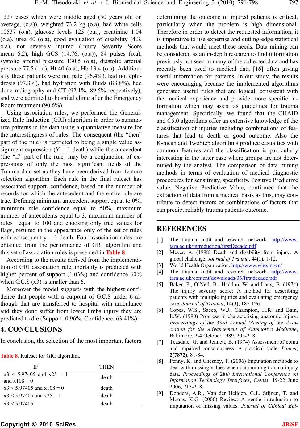

E.-M. Theodoraki et al. / J. Biomedical Science and Engineering 3 (2010) 791-798 797
1227 cases which were middle aged (50 years old on
average, (o.a)), weighted 73.2 kg (o.a), had white cells
10537 (o.a), glucose levels 125 (o.a), creatinine 1.04
(o.a), urea 40 (o.a), good evaluation of disability (4.3,
o.a), not severely injured (Injury Severity Score
mean=6.2), high GCS (14.76, (o.a)), 84 pulses (o.a),
systolic arterial pressure 130.5 (o.a), diastolic arterial
pressure 77.5 (o.a), Ht 40 (o.a), Hb 13.4 (o.a). Addition-
ally these patients were not pale (96.4%), had not ephi-
drosis (97.3%), had hydration with fluids (88.8%), had
done radiography and CT (92.1%, 89.5% respectively),
and were admitted to hosp ital clinic after the Emergency
Room treatment (90.6%).
Using association rules, we performed the General-
ized Rule Induction (GRI) algor ithm in order to summa-
rize patterns in the data using a quantitative measure for
the interestingness of rules. The consequent (the “then”
part of the rule) is restricted to being a single value as-
signment expression (Y = 1 death) while the antecedent
(the “if” part of the rule) may be a conjunction of ex-
pressions of only the most significant fields of the
Trauma data set as they have been derived from feature
selection algorithm. Each rule in the final ruleset has
associated support, confidence, based on the number of
records for which the antecedent and the entire rule are
true. Defining minimum antecedent support equal to 0%,
minimum rule confidence equal to 50%, maximum
number of antecedents equal to 3, maximum number of
rules equal to 100 and choosing only true values for
flags, resulted in the appearance only of the set of rules
with consequent y = 1 death. Four association rules are
obtained from the performance of GRI algorithm and
this set of association rules is presented in Table 8.
According to the results derived from the implementa-
tion of GRI association rule, mortality is predicted with
higher percent of support (1.03%) and confidence 60%
when G.C.S (x3) is smaller than 6.
Moreover the model suggests with the highest confi-
dence that people with a cutpoint of G.C.S under 6 al-
though that are transferred to hospital with ambulance
and they don't suffer from lower limbs injury they are
predicted to die (Support: 0.96%, Confidence: 63.41%).
4. CONCLUSIONS
In conclusion, the selection of the most important factors
Table 8. Ruleset for GRI algorithm.
IF THEN
x3 < 5.97405 and x25 = 1
and x108 = 0 death
x3 < 5.97405 and x108 = 0 death
x3 < 5.97405 and x25 = 1 death
x3 < 5.97405 death
determining the outcome of injured patients is critical,
particularly when the problem is high dimensional.
Therefore in order to detect the requested info rmation, it
is imperative to use expertise and cutting -edge statistical
methods that would meet these needs. Data mining can
be considered as an in-depth research to find information
previously not seen in many of the collected data and has
recently been used to medical data [16] often giving
useful information for patterns. In our study, the results
were encouraging because the implemented algorithms
generated useful rules that are logical, consistent with
the medical experience and provide more specific in-
formation which may assist as guidelines for trauma
management. Specifically, we found that the CHAID
and C5.0 algorith ms offer an extensive knowledg e of the
classification of injuries including combinations of fea-
tures that lead to death or good outcome. Also the
K-mean and TwoStep algorithms produce casualties with
common features and the classification is particularly
interesting in the latter case where groups are not deter-
mined by the analyst. The comparison of data mining
methods in terms of evaluation of medical diagnostic
procedures for sensitivity, specificity, Positive Predictive
value, Negative Predictive Value, confirmed that the
extraction of data from a medical basis as this, may con-
tribute to detect factors or combinations of factors that
can predict reliably trauma patients outcome.
REFERENCES
[1] The trauma audit and research network. http://www.
tarn.ac.uk/introduction/firstDecade.pdf
[2] Meyer, A. (1998) Death and disability from injury: A
global challenge. Journal of Trauma, 44(1), 1-12.
[3] World Health Organization. http://www.who.int/e n/
[4] The trauma audit and research network. http://www.
tarn.ac.uk/content/downloads/36/firstdecade.pdf
[5] Baker, P., O’Neil, B., Haddon, W. and Long, B. (1974)
The injury severity score: A method for describing
patients with multiple injuries and evaluating emergency
care. Journal of Trauma, 14(3), 187-196.
[6] Copes, W.S., Sacco, W.J., Champion, H.R. and Bain,
L.W. (1990) Progress in characterising anatomic injury.
Proceedings of the 33rd Annual Meeting of the Asso-
ciation for the Advancement of Automotive Medicine,
Baltimore, 2-4 October 1989, 205-218.
[7] Teasdale, G. and Jennett, B. (1974) Assessment of coma
and impaired consciousness. A practical scale. Lancet,
2(7872), 81-84.
[8] Penny, K. and Chesney, T. (2006) Imputation methods to
deal with missing values when data mining trauma injury
data. Proceedings of 28th International Conference on
Information Technology Interfaces, Cavtat, 19-22 June
2006, 213-218.
[9] Donders, A.R., Van der Heijden, G.J., Stijnen, T. and
Moons, K.G. (2006) Review: A gentle introduction to
imputation of missing values. Journal of Clinical Epi-

798 E.-M. Theodoraki et al. / J. Biomedical Science and Engineering 3 (2010) 791-798
demiology, 59(10), 1087-1091.
[10] Cox, D.R. and Hinkley, D.V. (1974) Theoretical statistics.
Chapman and Hall, London.
[11] Cramer, H. (1946) Mathematical methods of statistics.
Princeton University Press, Princeton.
[12] Dobson, A. (2002) An introduction to generalized linear
models. 2nd Edition, Chapman and Hall/CRC, London.
[13] Pearson, R.L. (1983) Karl Pearson and the chi-squared
test. International Statistical Review, 51, 59-72.
[14] Agrawal, R. and Srikant, R. (1994) Fast algorithms for
mining association rules. Proceedings of the 20th Inter-
national Conference on Very Large Databases, Santiago
de Chile, 12-15 September 1994, 479-499.
[15] Craven, P. and Wahba, G. (1979) Smoothing noisy data
with spline functions: Estimating the correct degree of
smoothing by the method of generalized cross-validation.
Numerische Mathematik, 31, 377-403.
[16] Breault, J.L., Goodall, C.R. and Fos, P.J. (2002) Data
mining a diabetic data warehouse. Artificial Intelligence
in Medicine, 26(1-2), 37-54.