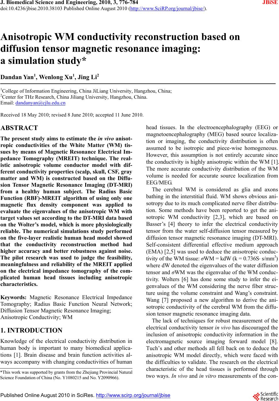J. Biomedical Science and Engineering, 2010, 3, 776-784 JBiSE
doi:10.4236/jbise.2010.38103 Published Online August 2010 (http://www.SciRP.org/journal/jbise/).
Published Online August 2010 in SciRes. http:// www. scirp. org/journal/jbise
Anisotropic WM conductivity reconstruction based on
diffusion tensor magnetic resonance imaging:
a simulation study*
Dandan Yan1, Wenlong Xu1, Jing Li2
1College of Information Engineering, China JiLiang University, Hangzhou, China;
2Center for THz Research, China Jiliang University, Hangzhou, China.
Received 18 May 2010; revised 8 June 2010; accepted 11 June 2010.
ABSTRACT
The present study aims to estimate the in vivo anisot-
ropic conductivities of the White Matter (WM) tis-
sues by means of Magnetic Resonance Electrical Im-
pedance Tomography (MREIT) technique. The real-
istic anisotropic volume conductor model with dif-
ferent conductivity properties (scalp, skull, CSF, gray
matter and WM) is constructed based on the Diffu-
sion Tensor Magnetic Resonance Imaging (DT-MRI)
from a healthy human subject. The Radius Basic
Function (RBF)-MREIT algorithm of using only one
magnetic flux density component was applied to
evaluate the eigenvalues of the anisotropic WM with
target values set according to the DT-MRI data based
on the Wolter’s model, which is more physiologically
reliable. The numerical simulations study performed
on the five-layer realistic human head model showed
that the conductivity reconstruction method had
higher accuracy and better robustness against noise.
The pilot research was used to judge the feasibility,
meaningfulness and reliability of the MREIT applied
on the electrical impedance tomography of the com-
plicated human head tissues including anisotropic
characteristics.
Keywords: Magnetic Resonance Electrical Impedance
Tomography; Radius Basic Function Neural Network;
Diffusion Tensor Magnetic Resonance Imaging;
Anisotropic Conductivity; WM
1. INTRODUCTION
Knowledge of the electrical conductivity distribution in
human body is important to many biomedical applica-
tions [1]. Brain disease and brain function activities al-
ways accompany with changing conductivities of human
head tissues. In the electroencephalography (EEG) or
magnetoencephalography (MEG) based source localiza-
tion or imaging, the conductivity distribution is often
assumed to be isotropic and piece-wise homogeneous.
However, this assumption is not entirely accurate since
the conductivity is highly anisotropic within the WM [1].
The more accurate conductivity distribution of the WM
volume is needed for accurate source localization from
EEG/MEG.
The cerebral WM is considered as glia and axons
bathing in the interstitial fluid. WM shows obvious ani-
sotropy due to its much complicated nerve fiber distribu-
tion. Some methods have been reported to get the ani-
sotropic WM conductivity [2,3], which are based on
Basser’s [4] theory to infer the electrical conductivity
tensor from the water self-diffusion tensor measured by
diffusion tensor magnetic resonance imaging (DT-MRI).
Self-consistent differential effective medium approach
(EMA) [2,5] was used to deduce the anisotropic conduc-
tivity of the WM tissue: σWM = kdW (k = 0.736S s/mm3)
where dW denoted the eigenvalues of the water diffusion
tensor and σWM was the eigenvalue of the WM conduc-
tivity. Wolters [6] has done some study to infer the ei-
genvalues of the WM considering the nerve fiber struc-
ture using the volume constraint and Wang’s constraint.
Wang [7] proposed a new algorithm to derive the ani-
sotropic conductivity of the cerebral WM from the diffu-
sion tensor magnetic resonance imaging data.
The lack of techniques for robust measurement of the
electrical conductivity tensor in vivo has discouraged the
inclusion of anisotropic conductivity information in the
electromagnetic source imaging forward model [8].
Tuch’s and other methods all fell back on to deduce the
anisotropic WM model directly, which were faced with
the difficulties to validate. The research on the electrical
characteristic of the head tissues is performed through
two ways. In vivo and in vitro measurements of the con-
*This work was supported by grants from the Zhejiang Provincial Natural
Science Foundation of China (No. Y1080215 and No. Y2090966).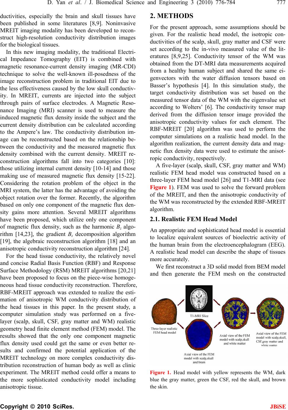

D. Yan et al. / J. Biomedical Science and Engineering 3 (2010) 776-784 777
ductivities, especially the brain and skull tissues have
been published in some literatures [8,9]. Noninvasive
MREIT imaging modality has been developed to recon-
struct high-resolution conductivity distribution images
for the biological tissues.
In this new imaging modality, the traditional Electri-
cal Impedance Tomography (EIT) is combined with
magnetic resonance-current density imaging (MR-CDI)
technique to solve the well-known ill-posedness of the
image reconstruction problem in traditional EIT due to
the less effectiveness caused by the low skull conductiv-
ity. In MREIT, currents are injected into the subject
through pairs of surface electrodes. A Magnetic Reso-
nance Imaging (MRI) scanner is used to measure the
induced magnetic flux density inside the subject and the
current density distribution can be calculated according
to the Ampere’s law. The conductivity distribution im-
age can be reconstructed based on the relationship be-
tween the conductivity and the measured magnetic flux
density combined with the current density. MREIT re-
construction algorithms fall into two categories [10]:
those utilizing internal current density [10-14] and those
making use of measured magnetic flux density [15-22].
Considering the rotation problem of the object in the
MRI system, the latter has the advantage of avoiding the
object rotation over the former. Recently, the algorithm
based on only one component of the magnetic flux den-
sity gains more attention. Several MREIT algorithms
have been proposed, which utilize only one component
of magnetic flux density, such as the harmonic Bz algo-
rithm [14,23], the gradient Bz decomposition algorithm
[19], the algebraic reconstruction algorithm [18] and an
anisotropic conductivity reconstruction algorithm [24].
For the head tissue conductivity, the relatively novel
and concise Radial Basis Function (RBF) and Response
Surface Methodology (RSM) MREIT algorithms [20,21]
have been proposed to focus on the piece-wise homoge-
neous head tissue conductivity reconstruction. Therefore,
RBF-MREIT approach was extended to realize the esti-
mation of anisotropic WM conductivity distribution of
the head tissues in this paper. In the present study, a
computer simulation study was performed on a five-
layer (scalp, skull, CSF, gray matter and WM) realistic
geometry head finite element method (FEM) model. The
results showed that the only one component magnetic
flux density used could get the same or even better re-
sults and confirmed the potential application of the
MREIT technology on more complex conductivity dis-
tribution reconstruction of human body as well as clinic
experiment. The MREIT method could offer a means to
the more sophisticated conductivity model including
anisotropic tissue.
2. METHODS
For the present approach, some assumptions should be
given. For the realistic head model, the isotropic con-
ductivities of the scalp, skull, gray matter and CSF were
set according to the in-vivo measured value of the lit-
eratures [8,9,25]. Conductivity tensor of the WM was
obtained from the DT-MRI data measurements acquired
from a healthy human subject and shared the same ei-
genvectors with the water diffusion tensors based on
Basser’s hypothesis [4]. In this simulation study, the
target conductivity distribution was set based on the
measured tensor data of the WM with the eigenvalue set
according to Wolters’ [6]. The conductivity tensor map
derived from the diffusion tensor image provided the
anisotropic conductivity values for each element. The
RBF-MREIT [20] algorithm was used to perform the
computer simulations on a realistic head model. In the
algorithm realization, the current density data and mag-
netic flux density data were used to estimate the anisot-
ropic conductivity, respectively.
A five-layer (scalp, skull, CSF, gray matter and WM)
realistic FEM head model was constructed based on a
three-layer FEM head model [26] and T1-MRI data (see
Figure 1). FEM was used to solve the forward problem
of the MREIT, and then the anisotropic conductivity of
the WM was reconstructed by the extended RBF-MREIT
algorithm.
2.1. Realistic FEM Head Model
An appropriate and sophisticated head model is essential
to localize equivalent sources of bioelectric activity of
the human brain from the electroencephalogram (EEG).
A realistic head model can describe the shape of tissues
more accurately.
We first reconstruct a 3D solid model from BEM model
and then generate the FEM mesh on the constructed
Figure 1. Head model with yellow represents the WM, dark
blue the gray matter, green the CSF, red the skull, and brown
the skin.

778 D. Yan et al. / J. Biomedical Science and Engineering 3 (2010) 776-784
3D model. The tissue interfaces are described by many
surface elements in the BEM model thus the 3D solid
model of tissue can be built simply by joining the sur-
face elements into a closed surface. Once given the 3D
solid model, the 3D FEM model can be obtained easily
by dividing the solid model of the tissue. A CAD soft-
ware Rhino and a FEM software ANSYS are used.
Based on the T1-weighted MRI data, a realistic five-
layer head model was constructed by FEM and boundary
element method (BEM) with 351386 quadratic tetrahe-
dral elements and 485767 nodes. ANSYS 10.0 was used
in the finite element modeling and the forward problem
calculation based on the EFM realistic head model.
The diffusion distribution of the conductivity could be
denoted by a 3 × 3 symmetric positive definite ma-
trix:











333231
232221
131211



 . When σ11 = σ22 = σ33 were con-
stants and other components were zero, the matrix could
be rendered as isotropic diffusion conductivity for the
grey matter and CSF tissues. For the anisotropic WM,
the diffusion distribution of the conductivities in each
element (voxel) of the FEM model were written as σ =
SΛWMST, where S = [S1 S
2 S 3] denoted the three unit
length orthogonal eigenvectors of the measured diffusion
tensor at the center of a WM finite element and ΛWM =










ltrans
ltrans
long



0 0
0 0
0 0
was the eigenvalue. λlong and λtrans
were the eigenvalue parallel (longitudinal) and perpen-
dicular (trans-verse) to the fiber directions, respectively.
The target conductivity distributions of the scalp, skull,
CSF, gray matter and WM were set according to the
measured data of corresponding tissues [9,25]. The WM
was set with anisotropic conductivity distribution based
on some existing measured data [2,6] and its anisotropic
characteristics.
2.2. Conductivity Reconstruction
MREIT imaging modality has been developed to recon-
struct high-resolution conductivity distribution images
for the biological issues. In this new imaging modality,
currents are injected into the subject through pairs of
surface electrodes. A Magnetic Resonance Imaging
(MRI) scanner is used to measure the induced magnetic
flux density B inside the subject and the current density
distribution J can be calculated according to the Am-
pere’s law. The conductivity distribution images can be
reconstructed based on the relationship between the
conductivity and the measured magnetic flux density
combined with the current density. MREIT is used to
image the conductivities of the human tissues, especially
in the human head. The advantages lie in that the mag-
netic signals tend to penetrate into the inner brain
through the low conductivity skull. MREIT reconstruc-
tion algorithms mainly fall into two categories: those
utilizing internal current density J and those making use
of only one component of measured magnetic flux den-
sity B. Due to the fact that only one component of the
magnetic flux density which parallels to the direction of
the main magnetic field of the MRI scanner can be
measured once, the rotation of the object is required，
which is impractical for MRI scanner. Considering the
rotation problem, the latter has the advantages over the
former of avoiding the object rotation dilemma. MREIT
algorithms that are based on current density require
knowledge of the magnetic flux density vector B = [Bx,
By, Bz].
MREIT reconstruction consists of the forward prob-
lem and the inverse problem. With given conductivity
and boundary condition, the calculation of peripheral
voltage values, current density distribution and/or mag-
netic flux density is referred to as the forward problem
of MREIT. The inverse problem deals with the recon-
struction of conductivity using the measured magnetic
flux density and computed current density information.
2.2.1. F or ward Problem
Under the quasi-static conditions, the relation between
the conductivity and the electrical potential U(r) induced
by the injected current is given by Poisson’s equation
together with the Neumann boundary conditions as:















elsewhere 0
electrodecurrent negativeon
electrodecurrent positiveon
,0
inj
inj
J
J
n
U
rrUr


(1)
where σ(r) is the electrical conductivity, Ω, the imaging
subject space, Jinj, the amount of injected current and

,
the gradient operator. For complex conductivity distribu-
tions, analytical solution to the forward problem ex-
pressed in Eq.1 does not exist. Therefore, a numerical
method must be applied. Finite element method (FEM)
is used to calculate the electrical potential and corre-
sponding magnetic flux density distribution for a given
conductivity distribution and boundary condition.
After obtaining the electric potential distribution U(r)
from solving Eq. 1 , the electric field and the interior cur-
rent density distribution are given as:
EJ
UE
 



(2)
Then the magnetic flux density can be calculated us-
ing the Biot-Savat law:

D. Yan et al. / J. Biomedical Science and Engineering 3 (2010) 776-784 779

0
3
() 4
rr
BrJ rdv
rr





 
 
 (3)
where B(r) is the magnetic flux density at the measure-
ment point, J(r’) the current density at the source point
and μ0 the magnetic permeability of the free space. In
order to avoid the singularity occurring when r = r’, B(r)
is treated as a node variable and J(r’) is used at the centre
of each finite element in Eq.3. The comparison between
the analytical solution and the numerical solution by
FEM method was performed [20,21] to indicate the fea-
sibility of solving the forward problem using the FEM.
2.2.2. Inverse Problem
For the inverse problem, the Radius Basic Function
(RBF) Neural Network system was used to seek the op-
timal estimation eigenvalues of the target conductivities:
λlong and λtrans of the WM, respectively. The conductivity
of the gray matter σGM and CSF σCSF were assumed to be
isotropic, thus each conductivity tensor has the same
value in three directions. The eigenvector data of each
element got from the DT-MRI measuring were com-
bined with the initial sample eigenvalues belong to a
certain range to perform the forward calculation. Based
on the sample data δ = {B, J} and the measured data “δ*
= {B*, J*}” from the forward calculation, the objection
function was set up and the RBF-MREIT algorithm was
used to reconstruct the anisotropic conductivity eigen-
values of the WM.
In the RBF-MREIT algorithm description, the rela-
tionship between the estimated target values [λlong
target,
λtrans
target] and the measured data “δ* = {B*, J*}” was con-
sidered as a “black box”. The Radius Basic Function
neural network was used herein to rebuild the input-
output relation system. After the system was trained by
the sample sets including the inputs and outputs couple
data, the optimal parameters of the system were found
through the optimization algorithm. Then the target val-
ues of the eigenvalues were reconstructed finally. There
were two processes in the realization of the RBF-
MREIT algorithm: the function set up and the function
optimization (See Figur e 2).
2.2.3. The Function Set Up
The inputs of the function were assumed as the sample
values of the unknown anisotropic eigenvalues [λlong, λtrans]
of the WM conductivity. The output was defined as the
objective function f(σ*, σ) between the measured data
“δ*={B*, J*}” and the computed sample data δ={B, J}.
22),()),(1(),(

  RECCf (4)
where CC(δ*, δ) and RE(δ*, δ) denoted the correlation
coefficient and relative error, respectively.
Five-layer
head
Model
22),()),(1()(

  RECCf
Figure 2. Flowchart of the RBF-MREIT algorithm frame.
2.2.4. The Function Optimization
Once the function between the input σ and the output f(σ)
is obtained, optimization method, herein the simplex
method, could be used to find the optimum point where
the objective function f(σ) is minimum and the measured
data “δ* = {B*, J*}” were most close to the computed
sample data set δ = {B, J} as well as the target σ* to the
estimated σ.
In conclusion, the inverse problem of the present
RBF-MREIT algorithm could be realized as follows:
Step 1: According to certain rules, some sampling input
points σ were chosen in the region of interest, and the
corresponding objective functions f(σ) were calculated
by solving the forward problem. Step 2: The sampling
input-output pairs were used to train the RBF network
and the trained RBF network function f(σ) was obtained.
Step 3: Estimating the optimum input parameter σi that
minimizes the output value using the simplex method.
Step 4: Resetting the region of interest by shrinking the
old region of interest to a new region and choosing the
optimum input parameters as the centre of the new re-
gion. Step 5: If the new region of interest was small
enough or‖σi+1 − σi≤‖ ε, then stop, otherwise, go to
step 1, where σi+1 and σi were the estimated conductivity
distribution at the (i + 1)th and ith iterations, respec-
tively, and ε was the allowable error.
3. SIMULATIOIN STUDY
In order to test the performance of RBF-MREIT algo-
rithm, numerical simulations were performed on a con-
centric five-layer human head model (consisting of the
scalp, skull, CSF, gray matter and WM) to estimate the
unknown anisotropic conductivity eigenvalues of the
WM. The results of the RBF-MREIT algorithm based on
different data δ were compared and analyzed.
3.1. Simulation Parameters
5mA bipolarity square-wave electric currents of 20Hz
frequency were injected into the head along the equator
of the head model as shown in Figure 3, which allowed
more signals flowing into the inner brain [20]. 7 elec-
trode pair positions were chosen to inject the current in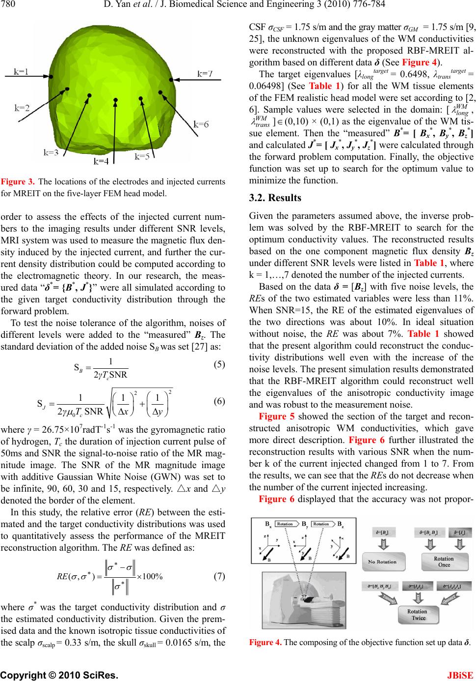

780 D. Yan et al. / J. Biomedical Science and Engineering 3 (2010) 776-784
Figure 3. The locations of the electrodes and injected currents
for MREIT on the five-layer FEM head model.
order to assess the effects of the injected current num-
bers to the imaging results under different SNR levels,
MRI system was used to measure the magnetic flux den-
sity induced by the injected current, and further the cur-
rent density distribution could be computed according to
the electromagnetic theory. In our research, the meas-
ured data “δ*= {B*, J*}” were all simulated according to
the given target conductivity distribution through the
forward problem.
To test the noise tolerance of the algorithm, noises of
different levels were added to the “measured” Bz. The
standard deviation of the added noise SB was set [27] as:
1
S2SNR
B
c
γT
 (5)
2
2
0
111
S2SNR
J
c
γTxy 



 



(6)
where γ = 26.75×107radT-1s-1 was the gyromagnetic ratio
of hydrogen, Tc the duration of injection current pulse of
50ms and SNR the signal-to-noise ratio of the MR mag-
nitude image. The SNR of the MR magnitude image
with additive Gaussian White Noise (GWN) was set to
be infinite, 90, 60, 30 and 15, respectively. △x and △y
denoted the border of the element.
In this study, the relative error (RE) between the esti-
mated and the target conductivity distributions was used
to quantitatively assess the performance of the MREIT
reconstruction algorithm. The RE was defined as:
%100),( 







RE (7)
where σ* was the target conductivity distribution and σ
the estimated conductivity distribution. Given the prem-
ised data and the known isotropic tissue conductivities of
the scalp σscalp = 0.33 s/m, the skull σskull = 0.0165 s/m, the
CSF σCSF = 1.75 s/m and the gray matter σGM = 1.75 s/m [9,
25], the unknown eigenvalues of the WM conductivities
were reconstructed with the proposed RBF-MREIT al-
gorithm based on different data δ (See Figure 4).
The target eigenvalues [λlong
target = 0.6498, λtrans target =
0.06498] (See Tab le 1) for all the WM tissue elements
of the FEM realistic head model were set according to [2,
6]. Sample values were selected in the domain: [WM
long
 ,
WM
trans
 ]

(0,10) × (0,1) as the eigenvalue of the WM tis-
sue element. Then the “measured” B*= [ B
x
*, B
y
*, B
z
*]
and calculated J*= [ Jx
*, Jy *, Jz *] were calculated through
the forward problem computation. Finally, the objective
function was set up to search for the optimum value to
minimize the function.
3.2. Results
Given the parameters assumed above, the inverse prob-
lem was solved by the RBF-MREIT to search for the
optimum conductivity values. The reconstructed results
based on the one component magnetic flux density Bz
under different SNR levels were listed in Table 1, where
k = 1,…,7 denoted the number of the injected currents.
Based on the data δ = [Bz] with five noise levels, the
REs of the two estimated variables were less than 11%.
When SNR=15, the RE of the estimated eigenvalues of
the two directions was about 10%. In ideal situation
without noise, the RE was about 7%. Table 1 showed
that the present algorithm could reconstruct the conduc-
tivity distributions well even with the increase of the
noise levels. The present simulation results demonstrated
that the RBF-MREIT algorithm could reconstruct well
the eigenvalues of the anisotropic conductivity image
and was robust to the measurement noise.
Figure 5 showed the section of the target and recon-
structed anisotropic WM conductivities, which gave
more direct description. Figure 6 further illustrated the
reconstruction results with various SNR when the num-
ber k of the current injected changed from 1 to 7. From
the results, we can see that the REs do not decrease when
the number of the current injected increasing.
Figure 6 displayed that the accuracy was not propor-
Figure 4. The composing of the objective function set up data δ.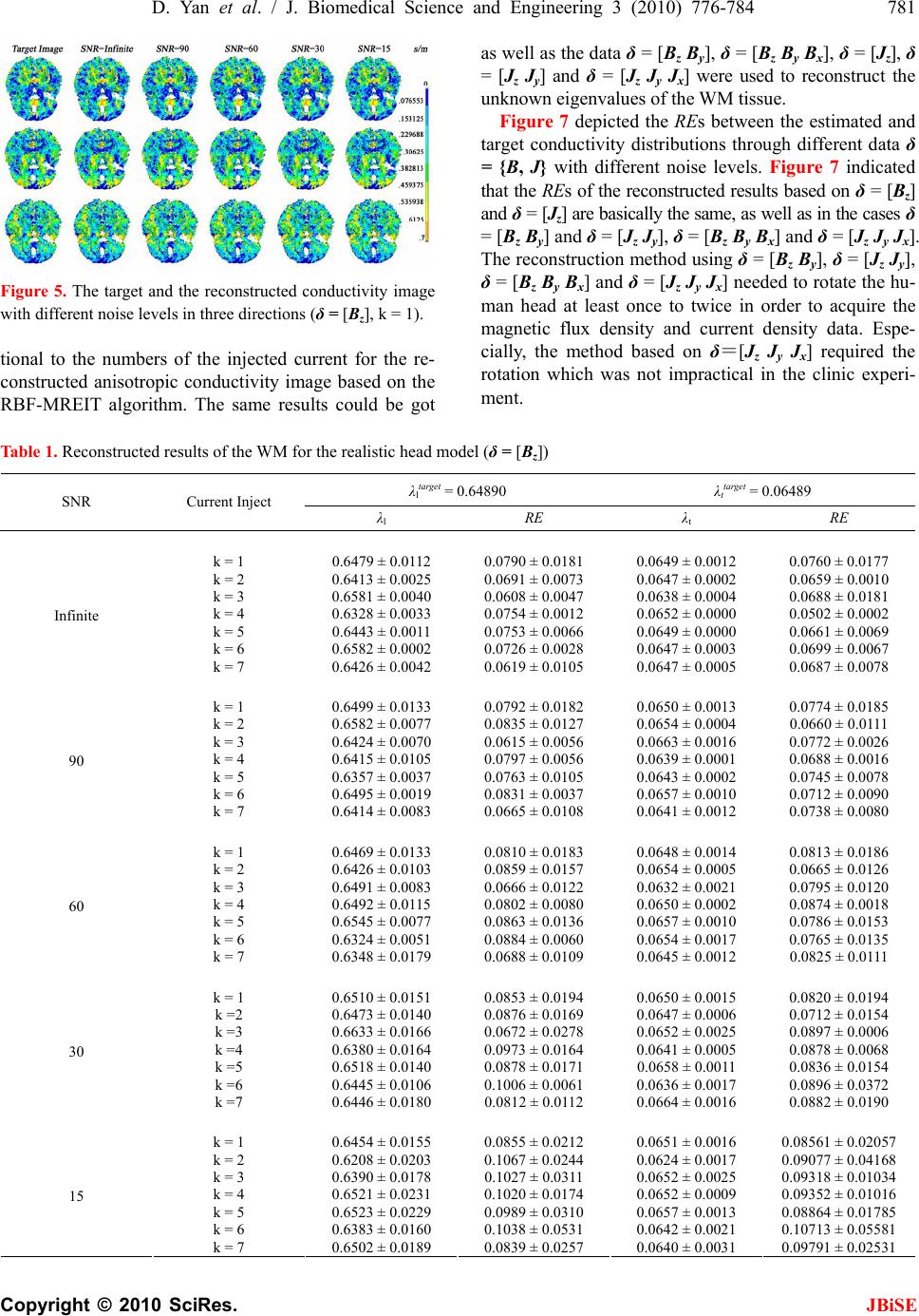

D. Yan et al. / J. Biomedical Science and Engineering 3 (2010) 776-784 781
Figure 5. The target and the reconstructed conductivity image
with different noise levels in three directions (δ = [Bz], k = 1).
tional to the numbers of the injected current for the re-
constructed anisotropic conductivity image based on the
RBF-MREIT algorithm. The same results could be got
as well as the data δ = [Bz By], δ = [Bz By Bx], δ = [Jz], δ
= [Jz J
y] and δ = [Jz J y J x] were used to reconstruct the
unknown eigenvalues of the WM tissue.
Figure 7 depicted the REs between the estimated and
target conductivity distributions through different data δ
= {B, J} with different noise levels. Figure 7 indicated
that the RE s of the reconstructed results based on δ = [Bz]
and δ = [Jz] are basically the same, as well as in the cases δ
= [Bz By] and δ = [Jz Jy], δ = [Bz By Bx] and δ = [Jz Jy Jx].
The reconstruction method using δ = [Bz By], δ = [Jz Jy],
δ = [Bz By Bx] and δ = [Jz Jy Jx] needed to rotate the hu-
man head at least once to twice in order to acquire the
magnetic flux density and current density data. Espe-
cially, the method based on δ＝[Jz J
y J x] required the
rotation which was not impractical in the clinic experi-
ment.
Table 1. Reconstructed results of the WM for the realistic head model (δ = [Bz])
λltarget = 0.64890 λttarget = 0.06489
SNR Current Inject
λl RE λt RE
k = 1 0.6479 ± 0.0112 0.0790 ± 0.0181 0.0649 ± 0.0012 0.0760 ± 0.0177
k = 2 0.6413 ± 0.0025 0.0691 ± 0.0073 0.0647 ± 0.0002 0.0659 ± 0.0010
k = 3 0.6581 ± 0.0040 0.0608 ± 0.0047 0.0638 ± 0.0004 0.0688 ± 0.0181
k = 4 0.6328 ± 0.0033 0.0754 ± 0.0012 0.0652 ± 0.0000 0.0502 ± 0.0002
k = 5 0.6443 ± 0.0011 0.0753 ± 0.0066 0.0649 ± 0.0000 0.0661 ± 0.0069
k = 6 0.6582 ± 0.0002 0.0726 ± 0.0028 0.0647 ± 0.0003 0.0699 ± 0.0067
Infinite
k = 7 0.6426 ± 0.0042 0.0619 ± 0.0105 0.0647 ± 0.0005 0.0687 ± 0.0078
k = 1 0.6499 ± 0.0133 0.0792 ± 0.0182 0.0650 ± 0.0013 0.0774 ± 0.0185
k = 2 0.6582 ± 0.0077 0.0835 ± 0.0127 0.0654 ± 0.0004 0.0660 ± 0.0111
k = 3 0.6424 ± 0.0070 0.0615 ± 0.0056 0.0663 ± 0.0016 0.0772 ± 0.0026
k = 4 0.6415 ± 0.0105 0.0797 ± 0.0056 0.0639 ± 0.0001 0.0688 ± 0.0016
k = 5 0.6357 ± 0.0037 0.0763 ± 0.0105 0.0643 ± 0.0002 0.0745 ± 0.0078
k = 6 0.6495 ± 0.0019 0.0831 ± 0.0037 0.0657 ± 0.0010 0.0712 ± 0.0090
90
k = 7 0.6414 ± 0.0083 0.0665 ± 0.0108 0.0641 ± 0.0012 0.0738 ± 0.0080
k = 1 0.6469 ± 0.0133 0.0810 ± 0.0183 0.0648 ± 0.0014 0.0813 ± 0.0186
k = 2 0.6426 ± 0.0103 0.0859 ± 0.0157 0.0654 ± 0.0005 0.0665 ± 0.0126
k = 3 0.6491 ± 0.0083 0.0666 ± 0.0122 0.0632 ± 0.0021 0.0795 ± 0.0120
k = 4 0.6492 ± 0.0115 0.0802 ± 0.0080 0.0650 ± 0.0002 0.0874 ± 0.0018
k = 5 0.6545 ± 0.0077 0.0863 ± 0.0136 0.0657 ± 0.0010 0.0786 ± 0.0153
k = 6 0.6324 ± 0.0051 0.0884 ± 0.0060 0.0654 ± 0.0017 0.0765 ± 0.0135
60
k = 7 0.6348 ± 0.0179 0.0688 ± 0.0109 0.0645 ± 0.0012 0.0825 ± 0.0111
k = 1 0.6510 ± 0.0151 0.0853 ± 0.0194 0.0650 ± 0.0015 0.0820 ± 0.0194
k =2 0.6473 ± 0.0140 0.0876 ± 0.0169 0.0647 ± 0.0006 0.0712 ± 0.0154
k =3 0.6633 ± 0.0166 0.0672 ± 0.0278 0.0652 ± 0.0025 0.0897 ± 0.0006
k =4 0.6380 ± 0.0164 0.0973 ± 0.0164 0.0641 ± 0.0005 0.0878 ± 0.0068
k =5 0.6518 ± 0.0140 0.0878 ± 0.0171 0.0658 ± 0.0011 0.0836 ± 0.0154
k =6 0.6445 ± 0.0106 0.1006 ± 0.0061 0.0636 ± 0.0017 0.0896 ± 0.0372
30
k =7 0.6446 ± 0.0180 0.0812 ± 0.0112 0.0664 ± 0.0016 0.0882 ± 0.0190
k = 1 0.6454 ± 0.0155 0.0855 ± 0.0212 0.0651 ± 0.0016 0.08561 ± 0.02057
k = 2 0.6208 ± 0.0203 0.1067 ± 0.0244 0.0624 ± 0.0017 0.09077 ± 0.04168
k = 3 0.6390 ± 0.0178 0.1027 ± 0.0311 0.0652 ± 0.0025 0.09318 ± 0.01034
k = 4 0.6521 ± 0.0231 0.1020 ± 0.0174 0.0652 ± 0.0009 0.09352 ± 0.01016
k = 5 0.6523 ± 0.0229 0.0989 ± 0.0310 0.0657 ± 0.0013 0.08864 ± 0.01785
k = 6 0.6383 ± 0.0160 0.1038 ± 0.0531 0.0642 ± 0.0021 0.10713 ± 0.05581
15
k = 7 0.6502 ± 0.0189 0.0839 ± 0.0257 0.0640 ± 0.0031 0.09791 ± 0.02531

782 D. Yan et al. / J. Biomedical Science and Engineering 3 (2010) 776-784
(a) λlong
(b) λtrans
Figure 6. The REs at different current injected numbers with
different noise levels (δ = [Bz]).
Comparing the REs of results based on δ = {B} with five
SNR noise levels, we can see that the REs using δ = [Bz]
were relatively smaller than the other two results using δ
= [Bz B
y] and δ = [Bz By Bx]. Even under the condition
that number k of the injected currents changed from 1 to
7, the same conclusion could be gained.
Figure 7 showed that the RBF-MREIT based on δ =
[Bz] could accurately detect the eigenvalues of the ani-
sotropic WM conductivity in the deep brain region. This
was a desired outcome of RBF-MREIT algorithm ap-
plied on the human head tissues. The RBF-MREIT algo-
rithm based on δ = [Bz] without rotation was practical in
further experimental study and provided a potential
means for reconstructing the complex conductivities of
the human brain and clinic application.
4. DISCUSSION
The RBF-MREIT algorithm, which was used to recon-
struct the piece-wise homogeneous conductivity of three
layer head model in [20], was extended to estimate the
eigenvalues of the WM. Viewed from the microscopic
angle, the conductivities of the human head are different
everywhere and anisotropic characteristic exists every-
where, even for the same tissue. Some research [6,28-30]
(a) λlong
(b) λtrans
Figure 7. The REs based on different data δ = {B, J} with
different noise levels (k = 1).
showed that the realistic head model with anisotropic
and inhomogeneous conductivity could improve the ac-
curacy of the source location in EEG/MEG analysis.
Presently, the MREIT algorithms [20,21] were used in
human head only under the condition of the piece-wise
homogeneous conductivities of the tissues. Some other
MREIT algorithms were not suitable to reconstruct the
conductivities of the complex head tissues.
RBF-MREIT algorithm based on one component
magnetic flux density solved the rotation problem in the
MREIT research and had strong usability in the future
clinic experiment. With different noise levels, all the REs
of the reconstructed WM based on one component mag-
netic flux density Bz were less than 11%, which was ac-
ceptable for the resolution requirement of the EEG/MEG
analysis. The simulation results suggested that the algo-
rithm was insensitive to the measurement noise. The
present simulation results demonstrated the feasibility of
the RBF-MREIT algorithm for anisotropic conductivity

D. Yan et al. / J. Biomedical Science and Engineering 3 (2010) 776-784 783
reconstruction of the human head tissues.
In summary, simulation results given above showed
that the RBF-MREIT algorithm [20] extended to detect
the eigenvalues of the anisotropic conductivity could
reconstruct anisotropic WM conductivity distribution of
the FEM human head model with high accuracy. The
target anisotropic conductivity of the WM was set up
based on the DT-MRI data according to the physical
experiment measurement performed on a healthy human
object. DT-MRI provides a noninvasive imaging modal-
ity to give more precise description of the human head
tissues with anisotropic characteristic. So in our simula-
tion, the head model considering the anisotropic tissues
and based on the DT-MRI was reliable.
The target anisotropic conductivity defined in our re-
search was based on Wolters’ model [3,6], in which the
eigenvalues of the anisotropic WM conductivity were
assumed to be homogeneous. The model set up by Tuch
[2,5] was more complicated than Wolters’, the eigenval-
ues of the anisotropic conductivity at every element be-
ing not identical. Wang [7] proposed a multi-com-
partment anisotropic WM model incorporating the par-
tial volume effects of the CSF and the intra-voxel fiber
crossing structure, which gave more refined description
through the physiology angle. All these models could be
the target values of the anisotropic conductivity recon-
struction for our next work.
The RBF-MREIT algorithm has certain limitations on
the application for the reconstruction of the inhomoge-
neous conductivities, especially on the complex human
head tissues. More unknown values will increase the
complexity and extend the training time of the Radius
Basic Function Neural Network for the inhomogeneous
conductivity reconstruction. All these will have impacts
on the accuracy and efficiency of the RBF-MREIT algo-
rithm. So the new MREIT algorithm, which is applied to
reconstruct the inhomogeneous conductivity including
the anisotropic conductivities of the human head tissue,
is our future research focus.
In the simulation, a current of 5 mA was used, which
is thought to be the upper safe limit for human beings
(IEC criterion). And for human head, it is a little higher.
So it would be desirable to utilize a better MRI scanner,
some denoising techniques and improved methods. The
information of the electrical properties of head tissues is
used for electroencephalographic source localization and
functional mapping of brain activities and functions. It
has been proved that the information about vivo tissue
conductivity values impacts the solution accuracy of
bioelectrical field problems [28-30]. In our future studies,
researches will focus on the study of continuous conduc-
tivity distribution reconstruction of the head tissues and
the experimental validation of the algorithm on the hu-
man head phantom experiment, as well as ways to re-
duce the amount of the injection current to less than
1mA for human security consideration in clinical ex-
periment.
5. CONCLUSIONS
We proposed the extended RBF-MREIT approach [20]
based on one component measured magnetic flux den-
sity to avoid the rotation procedure for the noninvasive
imaging of the three-dimensional conductivity distribu-
tion of the brain tissues with anisotropic characteristic.
In this paper, the FEM method was used to build a
five-layer head model constructed from DT-MRI data.
Simulations were performed on the FEM model to re-
construct the conductivities of anisotropic tissues. A se-
ries of computer simulation results demonstrate the fea-
sibility, the fast convergence ability and the improved
robustness against measurement noise of the algorithm.
Therefore, it is potential to provide a more accurate es-
timate of the WM anisotropic conductivity, and may
have important applications to neuroscience research or
clinical applications in neurology and neurophysiology.
However, the anisotropic conductivity estimation of
the WM tissue is more useful to obtain high resolution
source localization and mapping results. EEG/MEG in-
verse solution provides a unique tool to localize neural
electrical activity of a human brain from noninvasive
electromagnetic measurements. And it has been proved
that information about the vivo tissue conductivity val-
ues improves the solution accuracy of bioelectrical field
problems. Moreover, literatures [3, 6] show that the ani-
sotropic conductivities of the skull and WM may have
impact on EEG/MEG analysis and sensitivity of the
source location in the Early Left Anterior Negativity
(ELAN) usage of the language processing.
REFERENCES
[1] He, B. (2005) Neural engineering. Kluwer Academic
Publishers, Norwell.
[2] Haueisen, J., Tuch, D.S., Ramon, C., Schimpf, P.H.,
Wedeen, V.J., George, J.S. and Belliveau, J.W. (2002)
The influence of brain tissue anisotropy on human EEG
and MEG. NeuroImage, 15(1), 159-166.
[3] Wolters, C.H., Anwander, A., Tricoche, X., Weinstein,
D., Koch, M.A. and MacLeod, R.S. (2006) Influence of
tissue conductivity anisotropy on EEG/MEG field and
return current computation in a realistic head model: A
simulation and visualization study using high-resolution
finite element modeling. NeuroImage, 30(3), 813-826.
[4] Basser, P.J., Mattiello, J. and Lebihan, D. (1994) MR
diffusion tensor spectroscopy and imaging. Biophysical
Journal, 66(1), 259-267.
[5] Tuch, D.S., Wedeen, V.J., Dale, A.M., George, J.S. and
Belliveau, J.W. (1999) Conductivity tensor mapping of

784 D. Yan et al. / J. Biomedical Science and Engineering 3 (2010) 776-784
the human brain using diffusion MRI. Annals of the New
York Academy of Sciences, 888, 314-316.
[6] Wolters, C.H. (2002) Influence of tissue conductivity
inhomogeneity and anisotropy on EEG/MEG based
source localization in the human brain. Leipzig University,
Leipzig.
[7] Wang, K., Zhu, S.A., Mueller, B., Lim, K., Liu, Z.M. and
He, B. (2008) A new method to derive WM conductivity
from diffusion tensor MRI. IEEE Transactions on Bio-
medical Engineering, 55(10), 2481-2486.
[8] Goncalves, S., de Munck, J.C., Heethaar, R.M. and da
Silva, F.L. (2003) In vivo measurement of the brain and
skull resistivities using an EIT-based method and
realistic models for the head. IEEE Transactions on
Biomedical Engineering, 50(6), 754-767.
[9] Lai, Y., van Drongelen, W., Ding, L., Hecox, K.E.,
Towle, V.L., Frim, D.M. and He, B. (2005) Estimation of
in vivo human brain-to-skull conductivity ratio from
simultaneous extra- and intra-cranial electrical potential
recordings. Clinical Neurophysiology, 116(2), 456-465.
[10] Birgül, Ö., Eyüboğlu, B.M. and İder, Y.Z. (2003) Current
constrainted voltage scaled reconstruction (CCSVR)
algorithm for MR-EIT and its performance with different
probing current patterns. Physics in Medicine and Biology,
48, 653-671.
[11] İder, Y.Z. and Birgül, Ö. (1998) Use of the magnetic
field generated by the internal distribution of injected
currents for electrical impedance tomography (MR-EIT).
Elektrik, Turkish Journal of Electrical Engineering and
Computer Sciences, 6(3), 215-225.
[12] Khang, H.S., Lee, B.I., Oh, S.H., Woo, E.J., Lee, S.Y.,
Cho, M.H., Kwon, O., Yoon, J.R. and Seo, J.K. (2002)
J-substitution algorithm in magnetic resonance electrical
impedance tomography (MREIT): Phantom experiments
for static resistivity images. IEEE Transactions on Medi-
cal Imaging, 21(6), 695-702.
[13] Kwon, O., Lee, J.Y. and Yoo, J.R. (2002) Equipotential
line method for magnetic resonance electrical impedance
tomography (MREIT). Inverse Problems, 18(2), 1089-1100.
[14] Özdemir, M.S., Eyüboğlu, B.M. and Özbek, O. (2004)
Equipotential projection-based magnetic resonance elec-
trical impedance tomography and experimental realization.
Physics in Medicine and Biology, 49(20), 4765-4783.
[15] Seo, J.K., Yoon, J.R., Woo, E.J. and Kwon, O. (2003)
Reconstruction of conductivity and current density imaging
using only one component of magnetic field measure-
ments. IEEE Transactions on Biomedical Engineering,
50(9), 1121-1124.
[16] Oh, S.H., Lee, B.I., Woo, E.J., Lee, S.Y., Cho, M.H.,
Kwon, O. and Seo, J.K. (2003) Conductivity and current
density image reconstruction using harmonic Bz algori-
thm in magnetic resonance electrical impedance tomo-
graphy. Physics in Medicine and Biology, 48(19), 3101-
3116.
[17] Oh, S.H., Lee, B.I., Woo, E.J., Lee, S.Y., Kim, T.S.,
Kwon, O. and Seo, J.K. (2005) Electrical conductivity
images of biological tissue phantom in MREIT. Physi-
ological Measurement, 26(2), S279-S288.
[18] İder, Y.Z. and Onart, S. (2004) Algebric reconstruction
for 3D magnetic resonance-electrical impedance tomog-
raphy (MREIT) using one component of magnetic flux
density. Physiological Measurement, 25(1), 281-294.
[19] Park, C., Kwon, O., Woo, E.J. and Seo, J.K. (2004)
Electrical conductivity imaging using gradient Bz de-
composition algorithm in magnetic resonance electrical
impedance tomography (MREIT). IEEE Transactions on
Medical Imaging, 23(3), 388-394.
[20] Gao, N., Zhu, S.A. and He, B. (2005) Estimation of
electrical conductivity distribution within the human
head from magnetic flux density measurement. Physics in
Medicine and Biology, 50(11), 2675-2687.
[21] Gao, N., Zhu, S.A. and He, B. (2006) A new magnetic
resonance electrical impedance tomography (MREIT)
algorithm: the RSM-MREIT algorithm with applications
to estimation of human head conductivity. Physics in
Medicine and Biology, 51(12), 3067-3083.
[22] Gao, N. and He, B. (2008) Noninvasive imaging of
bioimpedance distribution by means of current recon-
struction magnetic resonance electrical impedance tomo-
graphy. IEEE Transactions on Biomedical Engineering,
55(5), 1530-1539.
[23] Birgül, Ö. and İder, Y.Z. (1998) Use of magnetic field
generated by the internal distribution of injected currents
for electrical impedance tomography (MREIT). Elektrik,
6(3), 215-225.
[24] Seo, J.K., Pyo, H.C., Park, C., Kwon, O. and Woo, E.J.
(2004) Image reconstruction of anisotropic conductivity
tensor distribution in MREIT: Computer simulation study.
Physics in Medicine and Biology, 49(18), 4371-4382.
[25] Zhang, Y.C., van Drongelen, W. and He, B. (2006)
Estimation of in vivo brain-to-skull conductivity ratio in
humans. Applied Physics Letters, 89(22), 223903-
2239033.
[26] Yao, Y., Zhu, S.A. and He, B. (2005) A method to derive
FEM models based on BEM models. IEEE 27th Annual
International Conference, Engineering in Medicine and
Biology Society (EMBS), Shanghai, 1-4 September 2005,
1575-1577.
[27] Scott, G.C., Joy, M.L.G. and Armstrong, R.L. (1992)
Sensitivity of magnetic-resonance current-density ima-
ging. Journal of Magnetic Resonance, 97(2), 235-254.
[28] Awada, K.A., Jackson, D.R., Baumann, S.B., Williams,
J.T., Wilton, D.R., Fink, P.W. and Prasky, B.R. (1998)
Effect of conductivity uncertainties and modeling errors
on EEG source localization using a 2-D model. IEEE
Transactions on Biomedical Engineering, 45(9), 1135-1145.
[29] Ferree, T.C., Eriksen, K.J. and Tucker, D.M. (2000)
Regional head tissue conductivity estimation for improved
EEG analysis. IEEE Transactions on Biomedical Engi-
neering, 47(12), 1584-1592.
[30] Gençer, N.G. and Acar, C.E. (2004) Sensitivity of EEG
and MEG measurements to tissue conductivity. Physics
in Medicine and Biology, 49(5), 707-717.