 Open Journal of Statistics, 2012, 2, 369-382 http://dx.doi.org/10.4236/ojs.2012.24045 Published Online October 2012 (http://www.SciRP.org/journal/ojs) Minimum Penalized Hellinger Distance for Model Selection in Small Samples Papa Ngom*, Bertrand Ntep Laboratoire de Mathematiques et Applications (LMA), Universite Cheikh Anta Diop, Dakar-Fann, Senegal Email: *papa.ngom@ucad.edu.sn, ntepjojo@yahoo.fr Received May 27, 2012; revised June 25, 2012; accepted July 10, 2012 ABSTRACT In statistical modeling area, the Akaike information criterion AIC, is a widely known and extensively used tool for model choice. The φ-divergence test statistic is a recently developed tool for statistical model selection. The popularity of the divergence criterion is however tempered by their known lack of robustness in small sample. In this paper the penalized minimum Hellinger distance type statistics are considered and some properties are established. The limit laws of the estimates and test statistics are given under both the null and the alternative hypotheses, and approximations of the power functions are deduced. A model selection criterion relative to these divergence measures are developed for parametric inference. Our interest is in the problem to testing for choosing between two models using some informa- tional type statistics, when independent sample are drawn from a discrete population. Here, we discuss the asymptotic properties and the performance of new procedure tests and investigate their small sample behavior. Keywords: Generalized Information; Estimation; Hypothesis Test; Monte Carlo Simulation 1. Introduction A comprehensive surveys on Pearson chi-square type statistics has been provided by many authors as Cochran [1], Watson [2] and Moore [3,4], in particular on quad- ratics forms in the cell frequencies. Recently, Andrews [5] has extended the Pearson chi-square testing method to non-dynamic parametric models, i.e., to models with covariates. Because Pearson chi-square statistics provide natural measures for the discrepancy between the ob- served data and a specific parametric model, they have also been used for discriminating among competing models. Such a situation is frequent in Social Sciences where many competing models are proposed to fit a giv- en sample. A well know difficulty is that each chi-square statistic tends to become large without an increase in its degrees of freedom as the sample size increases. As a consequence goodness-of-fit tests based on Pearson type chi-square statistics will generally reject the correct specification of every competing model. To circumvent such a difficulty, a popular method for model selection, which is similar to use of Akaike [6] Information Criterion (AIC), consists in considering that the lower the chi-square statistic, the better is the model. The preceding selection rule, however, does not take into account random variations inherent in the values of the statistics. We propose here a procedure for taking into account the stochastic nature of these differences so as to assess their significance. The main propose of this paper is to address this issue. We shall propose some convenient asymptotically standard normal tests for model selection based on φ-divergence type statistics. Following Vuong [7,8] the procedures considered here are testing the null hypothesis that the competing models are equally close to the data generating process (DGP) versus the alterna- tive hypothesis that one model is closer to the DGP where closeness of a model is measured according to the discrepancy implicit in the φ-divergence type statistic used. Thus the outcomes of our tests provide information on the strength of the statistical evidence for the choice of a model based on its goodness-of-fit (see Ngom [9]; Diedhiou and Ngom [10]). The model selection approach roposed here differs from those of Cox [11], and Akaike [12] for non nested hypotheses. This difference is that the present approach is based on the discrepancy implicit in the divergence type statistics used, while these other ap- proaches as Vuong’s [7] tests for model selection rely on the Kullback-Leibler [13] information criterion (KLIC). Beran [14] showed that by using the minimum Hellin- ger distance estimator, one can simultaneously obtain asymptotic efficiency and robustness properties in the presence of outliers. The works of Simpson [15] and *Corresponding author. C opyright © 2012 SciRes. OJS 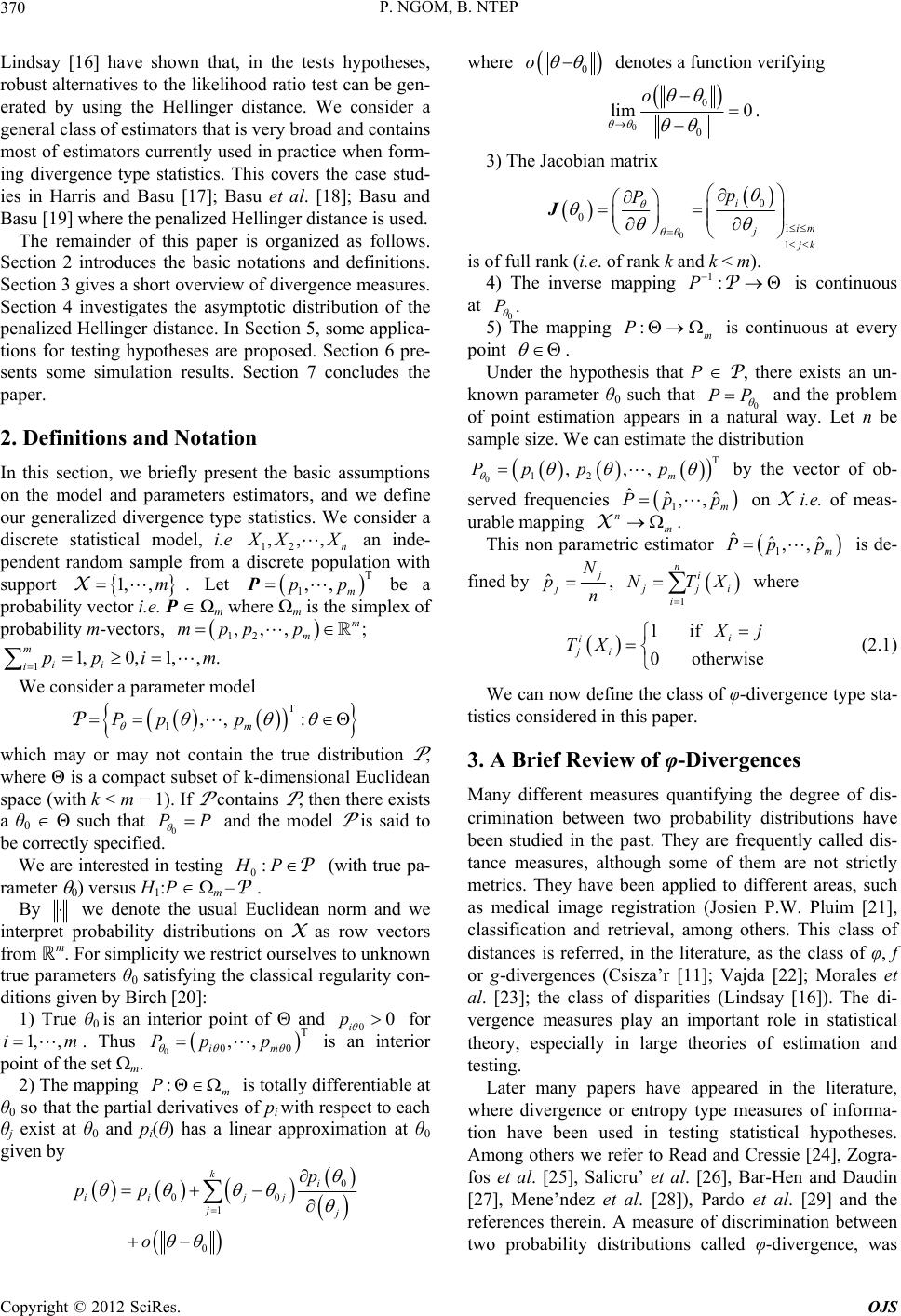 P. NGOM, B. NTEP 370 Lindsay [16] have shown that, in the tests hypotheses, robust alternatives to the likelihood ratio test can be gen- erated by using the Hellinger distance. We consider a general class of estimators that is very broad and contains most of estimators currently used in practice when form- ing divergence type statistics. This covers the case stud- ies in Harris and Basu [17]; Basu et al. [18]; Basu and Basu [19] where the penalized Hellinger distance is used. The remainder of this paper is organized as follows. Section 2 introduces the basic notations and definitions. Section 3 gives a short overview of divergence measures. Section 4 investigates the asymptotic distribution of the penalized Hellinger distance. In Section 5, some applica- tions for testing hypotheses are proposed. Section 6 pre- sents some simulation results. Section 7 concludes the paper. 2. Definitions and Notation In this section, we briefly present the basic assumptions on the model and parameters estimators, and we define our generalized divergence type statistics. We consider a discrete statistical model, i.e 12 n ,,, XX 1,X T 1,,pp , ; m m p T : PP 0:HPP an inde- pendent random sample from a discrete population with support . Let m be a probability vector i.e. P Ωm where Ωm is the simplex of probability m-vectors, ,m mp ,1,, .i m P 12 ,,p 1iii 1, m 0pp We consider a parameter model 1 ,, m Pp p P which may or may not contain the true distribution P , where Θ is a compact subset of k-dimensional Euclidean space (with k < m − 1). If P contains P , then there exists a θ0 Θ such that 0 and the model P is said to be correctly specified. We are interested in testing (with true pa- rameter 0) versus H1:P m –P. By 0p 1,i T 0m :P we denote the usual Euclidean norm and we interpret probability distributions on X as row vectors from ℝm. For simplicity we restrict ourselves to unknown true parameters θ0 satisfying the classical regularity con- ditions given by Birch [20]: 1) True θ0 is an interior point of and 0i for . Thus 0 is an interior point of the set m. ,mP 0 ,, i pp 2) The mapping m is totally differentiable at θ0 so that the partial derivatives of pi with respect to each θj exist at θ0 and pi(θ) has a linear approximation at θ0 given by 1 0 k ii j pp o 0 00 i jj j p where 0 o denotes a function verifying 0 0 0 lim 0 o . 3) The Jacobian matrix 01 0 0 1 i im j k p P J 1:PP .P is of full rank (i.e. of rank k and k < m). 4) The inverse mapping is continuous at 0 :m P 5) The mapping is continuous at every point PP . Under the hypothesis that P P, there exists an un- known parameter θ0 such that 0 0 T 12 , ,, m pPp p and the problem of point estimation appears in a natural way. Let n be sample size. We can estimate the distribution by the vector of ob- served frequencies 1 ˆˆ , ˆ,m ppP nX on X i.e. of meas- urable mapping . m This non parametric estimator 1 ˆˆ , ˆ,m ppP is de- fined by ˆj j pN n 1 n i i i jj NTX 1if 0 otherwise i i ji , where j TX (2.1) We can now define the class of φ-divergence type sta- tistics considered in this paper. 3. A Brief Review of φ-Divergences Many different measures quantifying the degree of dis- crimination between two probability distributions have been studied in the past. They are frequently called dis- tance measures, although some of them are not strictly metrics. They have been applied to different areas, such as medical image registration (Josien P.W. Pluim [21], classification and retrieval, among others. This class of distances is referred, in the literature, as the class of φ, f or g-divergences (Csisza’r [11]; Vajda [22]; Morales et al. [23]; the class of disparities (Lindsay [16]). The di- vergence measures play an important role in statistical theory, especially in large theories of estimation and testing. Later many papers have appeared in the literature, where divergence or entropy type measures of informa- tion have been used in testing statistical hypotheses. Among others we refer to Read and Cressie [24], Zogra- fos et al. [25], Salicru’ et al. [26], Bar-Hen and Daudin [27], Mene’ndez et al. [28]), Pardo et al. [29] and the references therein. A measure of discrimination between two probability distributions called φ-divergence, was Copyright © 2012 SciRes. OJS 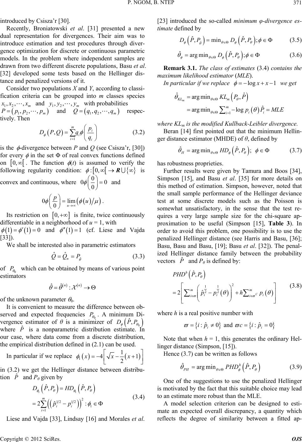 P. NGOM, B. NTEP 371 introduced by Csisza’r [30]. Recently, Broniatowski et al. [31] presented a new dual representation for divergences. Their aim was to introduce estimation and test procedures through diver- gence optimization for discrete or continuous parametric models. In the problem where independent samples are drawn from two different discrete populations, Basu et al. [32] developed some tests based on the Hellinger dis- tance and penalized versions of it. Consider two populations X and Y, according to classi- fication criteria can be grouped into m classes species 12 ,,, m xx 12 ,,, m Ppp p and with probabilities and respec- tively. Then 12 m Qq ,,,yy y 12 ,,, m q q 1 mi i i i , DPQ qq 0, (3.2) is the -divergence between P and Q (see Csisza’r, [30]) for every in the set Φ of real convex functions defined on . The function (t) is assumed to verify the following regularity condition: R:0, is convex and continuous, where 0 00 0 and lim u 0 0u p . Its restriction on 0, 11 is finite, twice continuously differentiable in a neighborhood of u = 1, with and 11 0 (cf. Liese and Vajda [33]). We shall be interested also in parametric estimators ˆ ˆˆ n QQ P P (3.3) of 0 which can be obtained by means of various point estimators : nn P ˆˆ of the unknown parameter 0. It is convenient to measure the difference between ob- served and expected frequencies 0 . A minimum Di- vergence estimator of θ is a minimizer of ˆ,DPP ˆ P0 where is a nonparametric distribution estimate. In our case, where data come from a discrete distribution, the empirical distribution defined in (2.1) can be used. In particular if we replace 1 41 2x ˆ P 1xx in (3.2) we get the Hellinger distance between distribu- tion and Pθ given by 11 1 2 12 : ˆ,DPP 1 1 2 ˆ 2 , ˆ m ii i DPP H pp (3.4) Liese and Vajda [33], Lindsay [16] and Morales et al. [23] introduced the so-called minimum φ-divergence es- timate defined by ˆΘ ˆˆ ,min ,;DPPDPP (3.5) Θ ˆˆ arg ;min, DPP log 1 (3.6) Remark 3.1. The class of estimates (3.4) contains the maximum likelihood estimator (MLE). In particular if we replace x 1 ˆˆ arg min, ˆ arg minlog m KL m m i ii KL P PMLp P E Θˆ arg ; ˆmin, HHDPP ˆ P we get where KLm is the modified Kullback-Leibler divergence. Beran [14] first pointed out that the minimum Hellin- ger distance estimator (MHDE) of θ, defined by (3.7) has robustness proprieties. Further results were given by Tamura and Boos [34], Simpson [15], and Basu et al. [35] for more details on this method of estimation. Simpson, however, noted that the small sample performance of the Hellinger deviance test at some discrete models such as the Poisson is somewhat unsatisfactory, in the sense that the test re- quires a very large sample size for the chi-square ap- proximation to be useful (Simpson [15], Table 3). In order to avoid this problem, one possibility is to use the penalized Hellinger distance (see Harris and Basu, [36]; Basu, Basu and Basu, [19]; Basu et al. [32]). The penal- ized Hellinger distance family between the probability vectors and Pθ is defined by: 2 11 22 ˆ, ˆ 2C mm ii i h i i PP p PH php D (3.8) where h is a real positive number with ˆˆ :0 and :0 ii ipc ip Note that when h = 1, this generates the ordinary Hel- linger distance (Simpson, [15]). Hence (3.7) can be written as follows Θ ˆmin ˆ arg , h PH DPPPH (3.9) One of the suggestions to use the penalized Hellinger is motivated by the fact that this suitable choice may lead to an estimate more robust than the MLE. A model selection criterion can be designed to esti- mate an expected overall discrepancy, a quantity which reflects the degree of similarity between a fitted ap- Copyright © 2012 SciRes. OJS 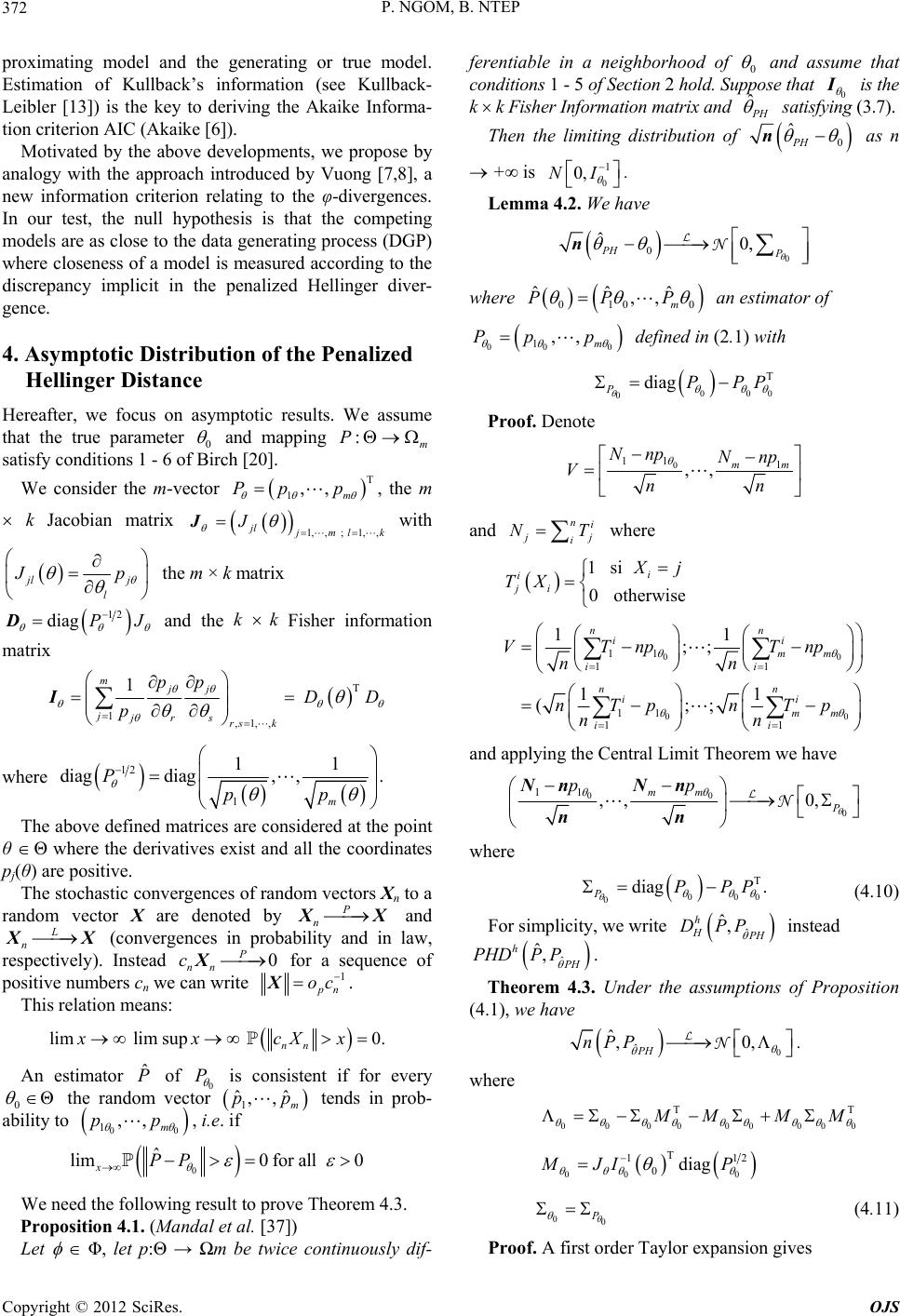 P. NGOM, B. NTEP 372 proximating model and the generating or true model. Estimation of Kullback’s information (see Kullback- Leibler [13]) is the key to deriving the Akaike Informa- tion criterion AIC (Akaike [6]). Motivated by the above developments, we propose by analogy with the approach introduced by Vuong [7,8], a new information criterion relating to the φ-divergences. In our test, the null hypothesis is that the competing models are as close to the data generating process (DGP) where closeness of a model is measured according to the discrepancy implicit in the penalized Hellinger diver- gence. 4. Asymptotic Distribution of the Penalized Hellinger Distance Hereafter, we focus on asymptotic results. We assume that the true parameter 0 and mapping :m P T 1,, m Pp p satisfy conditions 1 - 6 of Birch [20]. We consider the m-vector , the m k Jacobian matrix jl 1,, ; 1,, ml k J J with l jl j p the m × k matrix 12 diag PJ D and the k k Fisher information matrix T DD 1,1,, 1 mjj jjrs rs k pp p I where 12 1 diag diag, 11 , m Ppp P . The above defined matrices are considered at the point θ Θ where the derivatives exist and all the coordinates pj(θ) are positive. The stochastic convergences of random vectors Xn to a random vector X are denoted by n X L and n X c (convergences in probability and in law, respectively). Instead 0 P nn X for a sequence of positive numbers cn we can write 1 n oc X. This relation means: lim x lim sup x 0. nn cX x ˆ An estimator of 0 is consistent if for every 0Θ the random vector 1 tends in prob- ability to ˆ ,, ˆm pp 00 ,, m pp 1, i.e. if 0 ˆ lim0 for all0 xPP We need the following result to prove Theorem 4.3. Proposition 4.1. (Mandal et al. [37]) Let Φ, let p:Θ → Ωm be twice continuously dif- ferentiable in a neighborhood of 0 and assume that conditions 1 - 5 of Section 2 hold. Suppose that 0 I ˆ is the k k Fisher Information matrix and H satisfying (3.7). 0 ˆPH Then the limiting distribution of n 0 1 0,NI as n + is . Lemma 4.2. We have 0 0 ˆ0, PH P nN 010 0 ˆˆˆ ,, m PPP an estimator of where 00 0 1,, m Ppp defined in (2.1) with 000 0 T diag PPPP Proof. Denote 0 11 1 ,,mm Nnp Nnp Vnn ni jj i NT where and 1si 0otherwise j i i i j XT 00 00 11 11 11 11 11 ;; 11 (;; nn ii mm nn ii mm ii ii VTnp Tnp nn nTp nTp nn and applying the Central Limit Theorem we have 00 0 11 ,, 0, mm P pp NnN n nn N where 000 0 T diag . PPPP (4.10) ˆ ˆ, h H For simplicity, we write H DPP instead ˆ ˆ, h PH PHDPP . Theorem 4.3. Under the assumptions of Proposition (4.1), we have 0 ˆ ˆ,0, PH nPP N 00000000 0 TT . where MMM 00 0 T 1 0 12 diagMJI P 00 (4.11) Proof. A first order Taylor expansion gives Copyright © 2012 SciRes. OJS 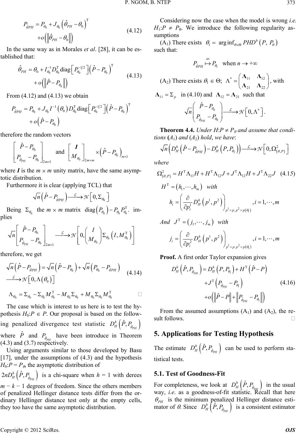 P. NGOM, B. NTEP 373 00 T 0 0 ˆPH J ˆ ˆ PH PH PP o (4.12) In the same way as in Morales et al. [28], it can be es- tablished that: 00 0 0 1T 0 ˆdiag ˆ PH ID P oPP 0 T 12 ˆ PP (4.13) From (4.12) and (4.13) we obtain 0 T 12 ˆ PPP ˆ ˆ PH PP 01 ˆ m PP 000 0 0 1T ˆ0diag ˆ PH PPJID oPP therefore the random vectors 0 021m PP 02mm M and I where I is the m m unity matrix, have the same asymp- totic distribution. Furthermore it is clear (applying TCL) that ˆ ˆPH nP P 0 0, N 0 Being 000 T PPP the m m matrix .diag im- plies 00 T ,nI M 0 0 0 ˆ21 ˆ 0, PH m PP I M PP N therefore, we get 0 ˆ 0 ˆ 0 ˆˆ 0, HPH nP P 00 0 TT nP PnP P N (4.14) 000000 MMM The case which is interest to us here is to test the hy- pothesis H0:P P. Our proposal is based on the follow- ing penalized divergence test statistic ˆ ˆ,PH h H DPP ˆ where and ˆPH have been introduce in Theorem (4.3) and (3.7) respectively. P ˆ ˆ,PH h H DPnP Θ1in arg,fh PHDPP Using arguments similar to those developed by Basu [17], under the assumptions of (4.3) and the hypothesis H0:P = P , the asymptotic distribution of 2 is a chi-square when h = 1 with derees m − k − 1 degrees of freedom. Since the others members of penalized Hellinger distance tests differ from the or- dinary Hellinger distance test only at the empty cells, they too have the same asymptotic distribution. Considering now the case when the model is wrong i.e. H1:P P. We introduce the following regularity as- sumptions (A1) There exists 1 ˆ as PH PP such that: 11 12 21 22 * ΛΛ ΛΛ 11 p when n + (A2) There exists 1 ; , with Λ1221 ΛΛ in (4.10) and such that 0 0 ˆ ˆ 0, PH PP PP n N. Theorem 4.4. Under H:P P and assume that condi- tions (A1) and (A2) hold, we have: 1 2 ˆ, ˆ,0, hh HH P PH nDP PDPP N 2TTTT 1112 1222 ,P where HH JJ HJJ (4.15) T 1,, m hh with 12 1 12 1 , ,,1,, h iH ippp p hDpp im p T 1,, m And jj with 121 12 2 . ,,1,, h iH ippp p jDpp im p Proof. A first order Taylor expansion gives 1 1 1 T ˆ T ˆ ˆ ˆˆ ,, ˆ PH PH PH hh HH DPPDPP HPP JP oP P PPP (4.16) From the assumed assumptions (A1) and (A2), the re- sult follows. 5. Applications for Testing Hypothesis The estimate ˆ ˆ,PH h H DPP ˆ ˆ, h H DPP can be used to perform sta- tistical tests. 5.1. Test of Goodness-Fit For completeness, we look at PH in the usual way, i.e. as a goodness-of-fit statistic. Recall that here H is the minimum penalized Hellinger distance esti- mator of . Since ˆ ˆ,PH h H DPP is a consistent estimator Copyright © 2012 SciRes. OJS  P. NGOM, B. NTEP 374 , h H DPP , the null hypothesis when using the statis- of tic is ˆ ˆ,PH h H DPP :,0 h oH PP HD or equivalently, Ho:P = P . Hence, if Ho is rejected so that one can infer that the parametric model P is misspecified. Since , h DPP H is non-negative and takes value zero only when P = P , the tests are defined through the critical region. ˆ, PH ˆ 2, PH h k PPq :,0 h oH PP CnD where q ,k is the (1 − )-quantile of the 2-distribution with m – k – 1 degrees of freedom. Remark 5.1. Theorem (4.4) can be used to give the following approximation to the power of test HD . Approximated power function is ˆ , ˆ 2, 12 h P n nDPP qn , , 2, PH Hk h kH P q DPP n (5.17) where q ,k is the (1 – )-quantile of the 2-distribution with m – k – 1 degrees of freedom and n is a sequence of distribution function tending uniformily to the stan- dard normal distribution . Note that if :,PP0 h oH , then for any fixed size the prob- ability of rejection HD :,0 h oH PP ˆ, 2, PH HD ˆ h with the rejec- tion rule k P q nD P tends to one as n . Obtaining the approximate sample n, guaranteeing a power for a give alternative P, is an interesting appli- cation of Formula (5.17). If we wish the power to be equal to *, we must solve the equation , h kH qD PP , , 1 1 2 P n n . It is not difficult to check that the sample size n*, is the solution of the following equation 2 2 2 21* , ,, 1 hh HH P nD PP n n DPP , , 2 2 k k q q The solution is given by 2 2 2, aab DPP 21 1 h H ab n with ,P and 2 a , h DPP ,kH bq and the required size is 01nn , where de- notes “integer part of”. 5.2. Test for Model Selection As we mentioned above, when one chooses a particular -divergence type statistic ˆˆ ˆˆ ,, PH PH hh HH DPP PHDPP ˆ with H the corresponding minimum penalized Hel- linger distance estimator of , one actually evaluates the goodness-of-fit of the parametric model P according to the discrepancy , h DPP H between the true distribu- tion P and the specified model P . Thus it is natural to define the best model among a collection of competing models to be the model that is closest to the true distribu- tion according to the discrepancy , h DPP H . In this paper we consider the problem of selecting be- tween two models. Let be another model, where is a q-dimensional parametric models P . In a similar way, we can define the minimum penalized Hellinger distance estimator of and the corresponding discrepancy (.|;GG , h DPG H for the model G . Our special interest is the situation in which a re- searcher has two competing parametric models P and G , and he wishes to select the better of two models based on their discrimination statistic between the observations and models P and G , defined respectively by ˆ, h DPP ˆPH H and ˆPH H Let the two competing parametric models P and G with the given discrepancy ˆ, h DPP ,. . h H DP . Définition 5.2. 0:,, eq hh HH DPP DPP means that the two models are equivalent, :, , hh H HDPPDPP pH means that P is better than G , :, , hh GHH DPP DPP means that P is worse than G . Remark 5.3. 1) It does not require that the same di- ˆ ˆ,PH h H DPP vergence type statistics be used in forming ˆ ˆ,PH h H DPP . Choosing, however, different dis- and crepancy for evaluating competing models is hardly juti- fied. 2) This definition does not require that either of the competing models be correctly specified. On the other hand, a correctly specified model must be at least as good as any other model. The following expression of the indicator ,, hh DPP DPP HH is unknown, but from the pre- vious section, it can be estimated by the difference ˆˆ ˆˆ ,, PH PH hh HH nD PPD PP This difference converges to zero under the null hypo- Copyright © 2012 SciRes. OJS  P. NGOM, B. NTEP 375 thesis 0 eq , but converges to a strictly negative or posi- tive constant when and G holds. Th justify the use of ˆPH PH H as a model selection indi- cator and common procedure of selecting the model with highest goodness-of-fit. ese properactually ˆ , h DPP ke into account t ˆ , h DPP ties ˆ ˆ , h H DPP As argued in the introduction, however, it is important to tahe random nature of the difference ˆPH PH H so as to assess its signific- ance. To do so we consider the asymptotic distribution ˆ ˆ , h H DPP of ˆ , PH h H P ˆ ˆˆ , PH h H nD PPD P 0 eq under . Our major task is to propose some tests for model se- lection, i.e. for the null hypothesis 0 eq against the al- ternative or G . We use the next lemma with ˆ H an d ˆ H as the corresponding minimum pena- lized Hellinger distance estimator of and . Using P and P defined earlier, we consider the vector T 1,, m kKk where 12 12 1 , with, h iH iPPP P kDPP p 1,, m i T 1,, m Qqq where 12 12 2 , w, h iH iPPPP qDPP p ith1,, m i Lemma 5.4. Under the assumptions of the Theorem (4.4), we have (i) for the model P ˆ T ˆ ,, 1 PH PH hh HH p DPP DP PQP o T ˆˆ ,P KPP T ˆˆ ,K PP ; (ii) for model G ˆ T ˆ ,, 1 PH PH hh HH p DPP DPG GQG o Proof. The results follow from a first order Taylor expan- sion. We define T 2; KQ QK KQQ 1 ˆ PH P PP P which is the variance of T ;KK QQ . Since K , K , Q , Q , and * are consistently estimated by their sample analogues ˆ K , ˆ K , ˆ Q , ˆ Q and *, hence 2 is consistently estimated by T 2 ˆˆˆˆˆ ˆˆ ˆ ˆ ˆ;; KQ QKKQ Q Next we define the model selection statistic and its asymptotic distribution under the null and alternative hypothesis. Let ˆˆ ˆˆ ,, ˆPH PH hh h HH n HIDP PDP P where HIh stands for the penalized Hellinger Indicator. The following theorem provides the limit distribution of HIh under the null and alternatives hypothesis. Theorem 5.5. Under the assumptions of Theorem (4.4), suppose that 0, then 001.,, eq h HHI N P H G H 1) Under the null hypothesis 2) Under the null hypothesis in probabil- ity. 3) Under the null hypothesis in prob- ability. Proof. From the Lemma (5.4), it follows that ˆˆ TT TT ˆˆ ˆˆ ,, ˆˆ ,, 1 PH PH PH PH hh HH hh HH p DPP DPP DPPDPGKPP KPP QP QGoPG 0: eq PG ˆˆ and Under H PH PG we get 1 ˆˆ TT TT ˆˆ T ˆˆ ,, ˆˆ 1 ;1 ˆ PH PH PH PH PH hh HH p p DPP DPP KPP KPP QP QPo P K P KQ QP P P o P Finally, applying the Central Limit Theorem and as- sumptions (A1) and (A2), we can now immediately obtain 0,1 . h HI N. 6. Computational Results 6.1. Example To illustrate the model procedure discussed in the pre- ceding section, we consider an example. We need to de- fine the competing models, the estimation method used for each competing model and the Hellinger penalized penalized type statistic to measure the departure of each proposed parametric model from the true data generating process. For our competing models, we consider the problem of choosing between the family of Poisson distribution and Copyright © 2012 SciRes. OJS 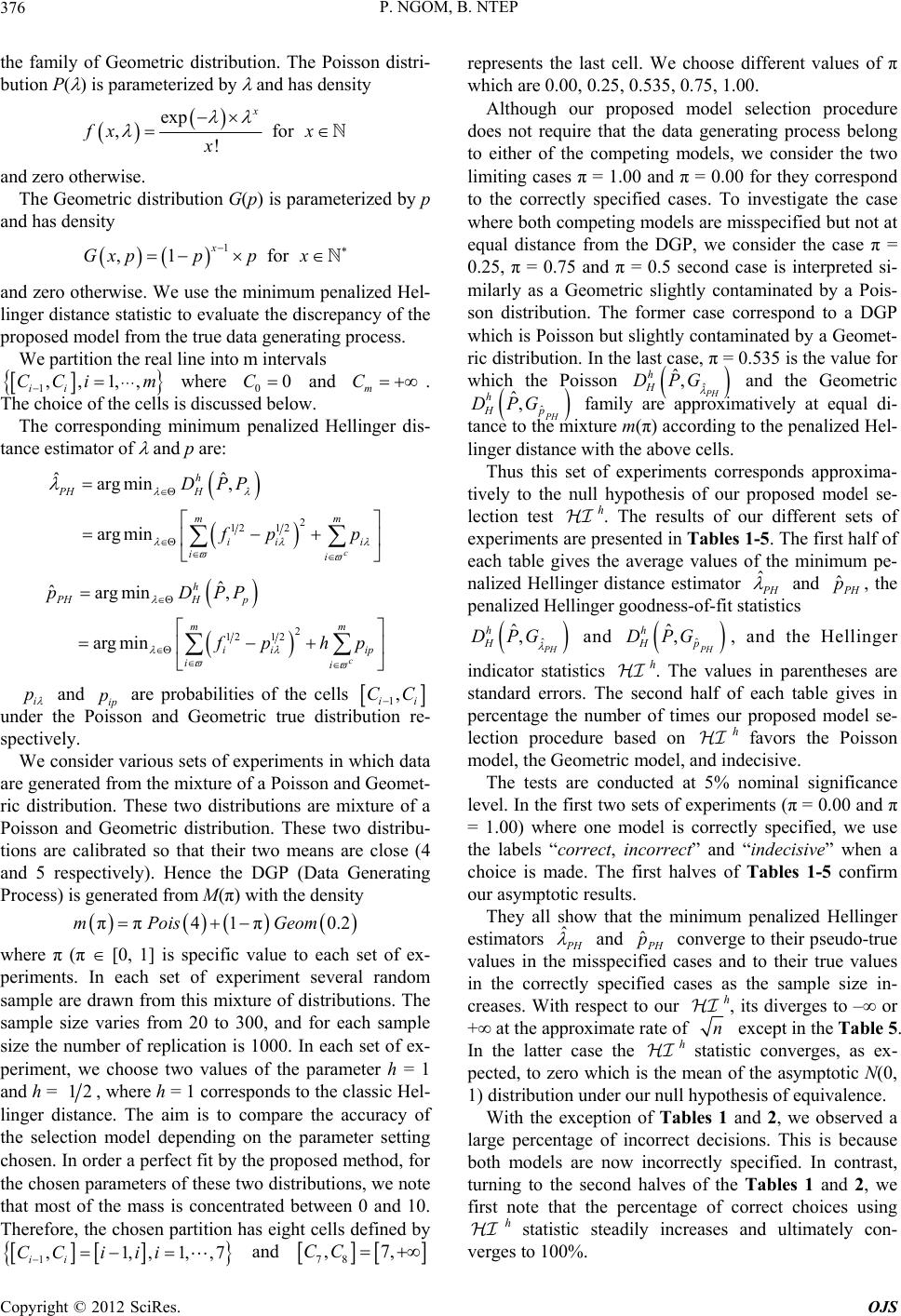 P. NGOM, B. NTEP 376 the family of Geometric distribution. The Poisson distri- bution P( ) is parameterized by and has density exp ! ,xx f for x x forpx and zero otherwise. The Geometric distribution G(p) is parameterized by p and has density 1 ,1 x Gxpp and zero otherwise. We use the minimum penalized Hel- linger distance statistic to evaluate the discrepancy of the proposed model from the true data generating process. We partition the real line into m intervals 1ii where 0 and ,,1iΛm C,,mCC 0C . The choice of the cells is discussed below. The corresponding minimum penalized Hellinger dis- tance estimator of and p are: 2 c m i i 12 12 ˆˆ arg min, argmin h PH H m ii i DPP pp 12 12 ˆ ˆarg min, argmin h PH H ii i p pDP 2 c mm ip i P php p i and ip are probabilities of the cells 1ii under the Poisson and Geometric true distribution re- spectively. ,CC We consider various sets of experiments in which data are generated from the mixture of a Poisson and Geomet- ric distribution. These two distributions are mixture of a Poisson and Geometric distribution. These two distribu- tions are calibrated so that their two means are close (4 and 5 respectively). Hence the DGP (Data Generating Process) is generated from M(π) with the density 0.2Geomππ 41πmPois where π (π [0, 1] is specific value to each set of ex- periments. In each set of experiment several random sample are drawn from this mixture of distributions. The sample size varies from 20 to 300, and for each sample size the number of replication is 1000. In each set of ex- periment, we choose two values of the parameter h = 1 and h = 12, where h = 1 corresponds to the classic Hel- linger distance. The aim is to compare the accuracy of the selection model depending on the parameter setting chosen. In order a perfect fit by the proposed method, for the chosen parameters of these two distributions, we note that most of the mass is concentrated between 0 and 10. Therefore, the chosen partition has eight cells defined by ,1,,7 1,1 ii CCi ,ii and 78 ,7,CC represents the last cell. We choose different values of π which are 0.00, 0.25, 0.535, 0.75, 1.00. Although our proposed model selection procedure does not require that the data generating process belong to either of the competing models, we consider the two limiting cases π = 1.00 and π = 0.00 for they correspond to the correctly specified cases. To investigate the case where both competing models are misspecified but not at equal distance from the DGP, we consider the case π = 0.25, π = 0.75 and π = 0.5 second case is interpreted si- milarly as a Geometric slightly contaminated by a Pois- son distribution. The former case correspond to a DGP which is Poisson but slightly contaminated by a Geomet- ric distribution. In the last case, π = 0.535 is the value for which the Poisson ˆ ˆ, h DPG PH H and the Geometric ˆPH Hp family are approximatively at equal di- tance to the mixture m(π) according to the penalized Hel- linger distance with the above cells. ˆ, h DPG ˆ Thus this set of experiments corresponds approxima- tively to the null hypothesis of our proposed model se- lection test h. The results of our different sets of experiments are presented in Tables 1-5. The first half of each table gives the average values of the minimum pe- nalized Hellinger distance estimator Hˆ and H p, the penalized Hellinger goodness-of-fit statistics ˆ ˆ,PH h H DPG and ˆ ˆ,PH h Hp DPG ˆ , and the Hellinger indicator statistics h. The values in parentheses are standard errors. The second half of each table gives in percentage the number of times our proposed model se- lection procedure based on h favors the Poisson model, the Geometric model, and indecisive. The tests are conducted at 5% nominal significance level. In the first two sets of experiments (π = 0.00 and π = 1.00) where one model is correctly specified, we use the labels “correct, incorrect” and “indecisive” when a choice is made. The first halves of Tables 1-5 confirm our asymptotic results. They all show that the minimum penalized Hellinger estimators H and ˆ H converge to their pseudo-true values in the misspecified cases and to their true values in the correctly specified cases as the sample size in- creases. With respect to our h, its diverges to – or + at the approximate rate of p n except in the Table 5. In the latter case the h statistic converges, as ex- pected, to zero which is the mean of the asymptotic N(0, 1) distribution under our null hypothesis of equivalence. With the exception of Tables 1 and 2, we observed a large percentage of incorrect decisions. This is because both models are now incorrectly specified. In contrast, turning to the second halves of the Tables 1 and 2, we first note that the percentage of correct choices using h statistic steadily increases and ultimately con- verges to 100%. Copyright © 2012 SciRes. OJS 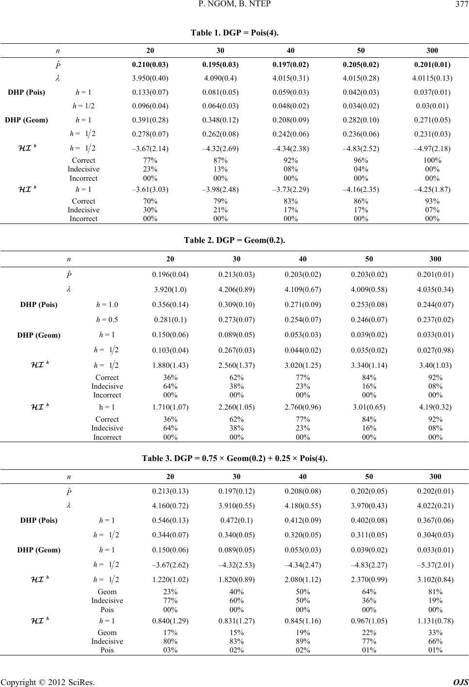 P. NGOM, B. NTEP Copyright © 2012 SciRes. OJS 377 Table 1. DGP = Pois(4). n 20 30 40 50 300 ˆ P 0.210(0.03) 0.195(0.03) 0.197(0.02) 0.205(0.02) 0.201(0.01) 3.950(0.40) 4.090(0.4) 4.015(0.31) 4.015(0.28) 4.0115(0.13) DHP (Pois) h = 1 0.133(0.07) 0.081(0.05) 0.059(0.03) 0.042(0.03) 0.037(0.01) h = 1/2 0.096(0.04) 0.064(0.03) 0.048(0.02) 0.034(0.02) 0.03(0.01) DHP (Geom) h = 1 0.391(0.28) 0.348(0.12) 0.208(0.09) 0.282(0.10) 0.271(0.05) h = 12 0.278(0.07) 0.262(0.08) 0.242(0.06) 0.236(0.06) 0.231(0.03) h h = 12 –3.67(2.14) –4.32(2.69) –4.34(2.38) –4.83(2.52) –4.97(2.18) Correct Indecisive Incorrect 77% 23% 00% 87% 13% 00% 92% 08% 00% 96% 04% 00% 100% 00% 00% h h = 1 –3.61(3.03) –3.98(2.48) –3.73(2.29) –4.16(2.35) –4.25(1.87) Correct Indecisive Incorrect 70% 30% 00% 79% 21% 00% 83% 17% 00% 86% 17% 00% 93% 07% 00% Table 2. DGP = Geom(0.2). n 20 30 40 50 300 ˆ P 0.196(0.04) 0.213(0.03) 0.203(0.02) 0.203(0.02) 0.201(0.01) 3.920(1.0) 4.206(0.89) 4.109(0.67) 4.009(0.58) 4.035(0.34) DHP (Pois) h = 1.0 0.356(0.14) 0.309(0.10) 0.271(0.09) 0.253(0.08) 0.244(0.07) h = 0.5 0.281(0.1) 0.273(0.07) 0.254(0.07) 0.246(0.07) 0.237(0.02) DHP (Geom) h = 1 0.150(0.06) 0.089(0.05) 0.053(0.03) 0.039(0.02) 0.033(0.01) h = 12 0.103(0.04) 0.267(0.03) 0.044(0.02) 0.035(0.02) 0.027(0.98) h h = 12 1.880(1.43) 2.560(1.37) 3.020(1.25) 3.340(1.14) 3.40(1.03) Correct Indecisive Incorrect 36% 64% 00% 62% 38% 00% 77% 23% 00% 84% 16% 00% 92% 08% 00% h h = 1 1.710(1.07) 2.260(1.05) 2.760(0.96) 3.01(0.65) 4.19(0.32) Correct Indecisive Incorrect 36% 64% 00% 62% 38% 00% 77% 23% 00% 84% 16% 00% 92% 08% 00% Table 3. DGP = 0.75 × Geom(0.2) + 0.25 × Pois(4). n 20 30 40 50 300 ˆ P 0.213(0.13) 0.197(0.12) 0.208(0.08) 0.202(0.05) 0.202(0.01) 4.160(0.72) 3.910(0.55) 4.180(0.55) 3.970(0.43) 4.022(0.21) DHP (Pois) h = 1 0.546(0.13) 0.472(0.1) 0.412(0.09) 0.402(0.08) 0.367(0.06) h = 12 0.344(0.07) 0.340(0.05) 0.320(0.05) 0.311(0.05) 0.304(0.03) DHP (Geom) h = 1 0.150(0.06) 0.089(0.05) 0.053(0.03) 0.039(0.02) 0.033(0.01) h = 12 –3.67(2.62) –4.32(2.53) –4.34(2.47) –4.83(2.27) –5.37(2.01) h h = 12 1.220(1.02) 1.820(0.89) 2.080(1.12) 2.370(0.99) 3.102(0.84) Geom Indecisive Pois 23% 77% 00% 40% 60% 00% 50% 50% 00% 64% 36% 00% 81% 19% 00% h h = 1 0.840(1.29) 0.831(1.27) 0.845(1.16) 0.967(1.05) 1.131(0.78) Geom Indecisive Pois 17% 80% 03% 15% 83% 02% 19% 89% 02% 22% 77% 01% 33% 66% 01% 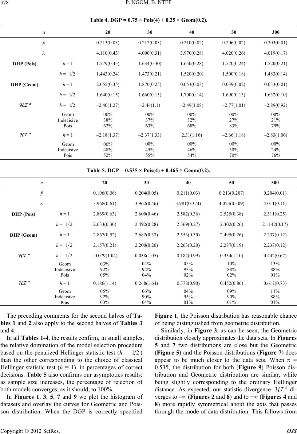 P. NGOM, B. NTEP 378 Table 4. DGP = 0.75 × Pois(4) + 0.25 × Geom(0.2). n 20 30 40 50 300 ˆ P 0.213(0.03) 0.212(0.03) 0.210(0.02) 0.206(0.02) 0.203(0.01) 4.110(0.43) 4.090(0.31) 3.970(0.28) 4.020(0.26) 4.019(0.17) DHP (Pois) h = 1 1.779(0.45) 1.634(0.30) 1.650(0.28) 1.570(0.24) 1.520(0.21) h = 12 1.443(0.24) 1.473(0.21) 1.520(0.20) 1.500(0.18) 1.483(0.14) DHP (Geom) h = 1 2.055(0.35) 1.870(0.25) 0.053(0.03) 0.039(0.02) 0.033(0.01) h = 12 1.640(0.15) 1.660(0.15) 1.700(0.14) 1.690(0.13) 1.632(0.10) h h = 12 –2.40(1.27) –2.44(1.1) –2.49(1.08) –2.77(1.01) –2.89(0.92) Geom Indecisive Pois 00% 38% 62% 00% 37% 63% 00% 32% 68% 00% 27% 83% 00% 21% 79% h h = 1 –2.18(1.37) –2.37(1.33) 2.31(1.16) –2.66(1.18) –2.83(1.06) Geom Indecisive Pois 00% 48% 52% 00% 45% 55% 00% 46% 54% 00% 30% 70% 00% 24% 76% Table 5. DGP = 0.535 × Pois(4) + 0.465 × Geom(0.2). n 20 30 40 50 300 ˆ P 0.196(0.06) 0.204(0.05) 0.211(0.03) 0.213(0.207) 0.204(0.01) 3.968(0.61) 3.962(0.46) 3.981(0.374) 4.023(0.309) 4.011(0.11) DHP (Pois) h = 1 2.869(0.63) 2.600(0.46) 2.582(0.36) 2.525(0.38) 2.311(0.25) h = 12 2.633(0.30) 2.492(0.28) 2.369(0.27) 2.302(0.26) 21.142(0.17) DHP (Geom) h = 1 2.867(0.52) 2.682(0.37) 2.553(0.30) 2.495(0.26) 2.237(0.12) h = 12 2.157(0.21) 2.200(0.20) 2.263(0.20) 2.287(0.19) 2.237(0.12) h h = 12 –0.079(1.04) 0.038(1.05) 0.182(0.99) 0.334(1.10) 0.442(0.67) Geom Indecisive Pois 03% 92% 05% 04% 92% 04% 05% 93% 02% 10% 88% 02% 13% 88% 01% h h = 1 0.186(1.14) 0.248(1.64) 0.378(0.90) 0.452(0.86) 0.617(0.73) Geom Indecisive Pois 05% 92% 03% 06% 90% 04% 04% 95% 01% 09% 90% 01% 11% 88% 01% The preceding comments for the second halves of Ta- bles 1 and 2 also apply to the second halves of Tables 3 and 4. In all Tables 1-4, the results confirm, in small samples, the relative domination of the model selection procedure based on the penalized Hellinger statistic test (h = 12 ) than the other corresponding to the choice of classical Hellinger statistic test (h = 1), in percentages of correct decisions. Table 5 also confirms our asymptotics results: as sample size increases, the percentage of rejection of both models converges, as it should, to 100%. In Figures 1, 3, 5, 7 and 9 we plot the histogram of datasets and overlay the curves for Geometric and Pois- son distribution. When the DGP is correctly specified Figure 1, the Poisson distribution has reasonable chance of being distinguished from geometric distribution. Similarly, in Figure 3, as can be seen, the Geometric distribution closely approximates the data sets. In Figures 5 and 7 two distributions are close but the Geometric (Figure 5) and the Poisson distributions (Figure 7) does appear to be much closer to the data sets. When = 0.535, the distribution for both (Figure 9) Poisson dis- tribution and Geometric distribution are similar, while being slightly corresponding to the ordinary Hellinger distance. As expected, our statistic divergence h di- verges to – (Figures 2 and 8) and to + (Figures 4 and 8) more rapidly symmetrical about the axis that passes through the mode of data distribution. This follows from Copyright © 2012 SciRes. OJS  P. NGOM, B. NTEP 379 Figure 1. Histogram of DGP Pois(4) with n = 50. Figure 2. Comparative barplot of h depending n. Figure 3. Histogram of DGP-Geom(0.2) with n = 50. Figure 4. Comparaison barplot of h depending n. Figure 5. Histogram of DGP = 0.75 “Geom + 0.25” Pois with n = 50. the fact that these two distributions are equidistant from the fact that these two distributions are equidistant from the DGP and would be difficult to distinguish from data in practice. The preceding results in tables and the Theorem (5.5) confirm, in Figures 2, 4, 6 and 8, that the Hellinger indi- cator for the model selection procedure based on panel- ized hellinger divergence statistic with h = 0.5 (light bars) dominates the procedure obtained with h = 1 (dark bars) when we use the penalized Hellinger distance test than the classical Hellinger distance test. Hence, Figure 10 allows a comparison with the asymptotic (0, 1) ap- proximation under our null hypothesis of equivalence. Hence the indicator 1/2, based on the penalized Hel- linger distance is closer to the mean of (0, 1) than is the indicator 1. N N Copyright © 2012 SciRes. OJS  P. NGOM, B. NTEP 380 Figure 6. Comparative barplot of h depending n. Figure 7. Histogram of DGP = 0.25 × “Geom + 0.75” Pois with n = 50. Figure 8. Comparative barplot of h. Figure 9. Histogram of DGP = 0.465 “Geom + 0.535” Pois with n = 50. Figure 10. Comparative barplot of h depending n. 7. Conclusion In this paper we investigated the problems of model se- lection using divergence type statistics. Specifically, we proposed some asymptotically standard normal and chi-square tests for model selection based on divergence type statistics that use the corresponding minimum pe- nalized Hellinger estimator. Our tests are based on test- ing whether the competing models are equally close to the true distribution against the alternative hypotheses that one model is closer than the other where closeness of a model is measured according to the discrepancy im- plicit in the divergence type statistics used. The penalized Hellinger divergence criterion outperforms classical cri- teria for model selection based on the ordinary Hellinger distance, especially in small sample, the difference is Copyright © 2012 SciRes. OJS  P. NGOM, B. NTEP 381 expected to be minimal for large sample size. Our work can be extended in several directions. One extension is to use random instead of fixed cells. Random cells arise when the boundaries of each cell ci depend on some un- known parameter vector , which are estimated. For various examples, see e.g., Andrews [37]. For instance, with appropriate random cells, the asymptotic distribu- tion of a Pearson type statistic may become independent of the true parameter o under correct specification. In view of this latter result, it is expected that our model selection test based on penalized Hellinger divergence measures will remain asymptotically normally or chi- square distributed. 8. Acknowledgements This research was supported, in part, by grants from AIMS (African Institute for Mathematical Sciences) 6 Melrose Road, Muizenberg-Cape Town 7945 South Af- rica. REFERENCES [1] W. G. Cochran, “The 2 Test of Goodness of Fit,” The Annals of Mathematical Statistics, Vol. 23, No. 3, 1952, pp. 315-345. doi:10.1214/aoms/1177729380 [2] G. S. Watson, “On the Construction of Significance Tests on the Circle and the Sphere,” Biometrika, Vol. 43, No. 3-4, 1956, pp. 344-352. doi:10.2307/2332913 [3] D. S. Moore, “Chi-Square Tests in Studies in Statistics,” 1978. [4] D. S. Moore, “Tests of Chi-Squared Type Goodness of Fit Techniques,” 1986. [5] D. W. K. Andrews, “Chi-Square Diagnostic Tests for Eco- nometric Models: Theory,” Econometrica, Vol. 56, No. 6, 1988, pp. 1419-1453. doi:10.2307/1913105 [6] H. A. Kaike, “Information Theory and Extension of the Likelihood Ratio Principle,” Proceedings of the Second International Symposium of Information Theory, 1973, pp. 257-281. [7] Q. H. Vuong, “Likelihood Ratio Tests for Model Selec- tion and Non-Nested Hypotheses,” Econometrika, Vol. 57, No. 2, 1989, pp. 257-306. doi:10.2307/1912557 [8] Q. H. Vuong and W. Wang, “Minimum Chi-Square Es- timation and Tests for Model Selection,” Journal of Econo- metrics, Vol. 57, No. 1-2, 1993, pp. 141-168. doi:10.1016/0304-4076(93)90104-D [9] P. Ngom, “Selected Estimated Models with Á-Divergence Statistics Global,” Journal of Pure and Applied Mathe- matics, Vol. 3, No. 1, 2007, pp. 47-61. [10] A. Diédhiou and P. Ngom, “Cutoff Time Based on Gen- eralized Divergence Measure,” Statistics and Probability Letters, Vol. 79, No. 10, 2009, pp. 1343-1350. doi:10.1016/j.spl.2009.02.006 [11] D. R. Cox, “Tests of Separate Families of Hypotheses,” Proceedings of the Fourth Berkeley Symposium on Mathe- matical Statistics and Probability, Los Angeles, 20-30 June 1961, pp. 105-123. [12] H. Akaike, “A New Look at the Statistical Model Identi- fication,” IEEE Transaction on Information Theory, Vol. 19, No. 6, 1974, pp. 716-723. [13] S. Kullback and R. A. Leibler, “On Information and Suf- ficiency,” The Annals of Mathematical Statistics, Vol. 22, No. 1, 1951, pp. 79-86. doi:10.1214/aoms/1177729694 [14] R. J. Bearn, “Minimum Hellinger Distance Estimates for Parametric Models,” The Annals of Mathematical Statis- tics, Vol. 5, No. 3, 1977, pp. 445-463. [15] D. G. Simpson, “Hellinger Deviance Test: Efficiency, Breakdown Points and Examples,” Journal of American Statistical Association, Vol. 84, No. 405, 1989, pp. 107- 113. doi:10.1080/01621459.1989.10478744 [16] B. G. Lindsay, “Efficiency versus Robustness: The Case for Minimum Distance Hellinger Distance and Related Methods,” Annals of Statistics, Vol. 22, No. 2, 1994, pp. 1081-1114. doi:10.1214/aos/1176325512 [17] A. Basu and B. G. Lindsay, “Minimum Disparity Estima- tion for Continuous Models: Efficiency, Distributions and Robustness,” The Annals of Mathematical Statistics, Vol. 46, No. 4, 1994, pp. 683-705. doi:10.1007/BF00773476 [18] A. Basu, I. R. Harris and S. Basu, “Tests of Hypotheses in Discrete Models Based on the Penalized Hellinger Dis- tance,” Statistics and Probability Letters, Vol. 27, No. 4, 1996, pp. 367-373. doi:10.1016/0167-7152(95)00101-8 [19] A. Basu and S. Basu, “Penalized Minimum Disparity Methods for Multinomial Models,” Statistica Sinica, Vol. 8, 1998, pp. 841-860. [20] M. W. Birch, “The Detection of Partial Association, II: The General Case,” Journal of the Royal Statistical So- ciety, Vol. 27, No. 1, 1965, pp. 111-124. [21] J. P. W. Pluim, J. B. A. Maintz and A. M. Viergever, “f-Information Measures to Medical Image Registration,” IEEE Transactions on Medical Imaging, Vol. 23, No. 12, 2004, pp. 1508-1516. doi:10.1109/TMI.2004.836872 [22] I. Vajda, “Theory of Statistical Evidence and Informa- tion,” Kluwe Academic Plubisher, Dordrecht, 1989. [23] D. Morales, L. Pardo and I. Vajda, “Asymptotic Diver- gence of Estimates of Discrete Distribution,” Journal of Statistical Planning and Inference, Vol. 483, No. 3, 1995, pp. 347-369. doi:10.1016/0378-3758(95)00013-Y [24] N. Cressie and T. R. C. Read, “Multinomial Goodness of Fit Test,” Journal of the Royal Statistical Society, Vol. 463, No. 3, 1984, pp. 440-464. [25] K. Zografos and K. Ferentinos, “Divergence Statistics Sampling Properties and Multinomial Goodness of fit and Divergence Tests,” Communications in Statistics—Theory and Methods, Vol. 19, No. 5, 1990, pp. 1785-1802. doi:10.1080/03610929008830290 [26] M. Salicru, D. Morales, M. L. Menendez, et al., “On the Applications of Divergence Type Measures in Testing Statistical Hypotheses,” Journal of Multivariate Analysis, Vol. 51, No. 2, 1994, pp. 372-391. doi:10.1006/jmva.1994.1068 [27] A. Bar-Hen and J. J. Dandin, “Generalisation of the Ma- Copyright © 2012 SciRes. OJS  P. NGOM, B. NTEP Copyright © 2012 SciRes. OJS 382 halanobis Distance in the Mixed Case,” Journal of Mul- tivariate Analysis, Vol. 532, No. 2, 1995, pp. 332-342. doi:10.1006/jmva.1995.1040 [2] L. Pardo, D. Mmorales, M. Salicrù and M. L. Menendez, “Generalized Divergences Measures: Amount of Infor- mation, Asymptotic-Distribution and Its Applications to Test Statistical Hypotheses,” International Sciences, Vol. 84, No. 3-4, 1995, pp. 181-198. [3] M. L. Menendez, L. Pardo, M. Salicrù and D. Morales, “Divergence Measures, Based on Entropy Functions and Statistical Inference,” Sankyã: The Indian Journal of Sta- tistics, Vol. 57, No. 3, 1995, pp. 315-337. [4] I. Csiszár, “Information-Type Measure of Difference of Probability Distribution and Indirect Observations,” Studia Scientiarum Mathematicarum Hungarica, Vol. 2, 1967, pp. 299-318. [5] M. Broniatowski and A. Toma, “Dual Divergence Esti- mators and Tests: Robustness Results,” Journal of Multi- variate Analysis, Vol. 102, No. 1, 2011, pp. 20-36. [6] A. Basu, A. Mandal and L. Pardo, “Hypothesis Testing for Two Discrete Populations Based on the Hellinger Dis- tance,” Statistics and Probability Letters, Vol. 80, No. 3-4, 2010, pp. 206-214. doi:10.1016/j.spl.2009.10.008 [7] F. Liese and I. Vajda, “Convex Statistical Distance, vol. 95 of Teubner-Texte zur Mathematik,” 1987. [8] R. Tamura and D. D. Boos, “Minimum Hellinger Dis- tance Estimation for Multivariate Location and Covari- ance,” Journal of American Statistical Association, Vol. 81, No. 333, 1989, pp. 223-229. [9] A. Basu, S. Sarkar and A. N. Vidyashankar, “Minimum Negative Exponential Disparity Estimation in Parametric Models,” Journal of Statistical Planning and Inference, Vol. 582, No. 2, 1997, pp. 349-370. doi:10.1016/S0378-3758(96)00078-X [10] I. R. Harris and A. Basu, “Hellinger Distance as Pena- lized Loglikelihood,” Communications in Statistics— Theory and Methods, Vol. 21, No. 3, 1994, pp. 637-646. doi:10.1080/03610929208830804 [11] A. Mandal, R. K. Patra and A. Basu, “Minimum Hellin- ger Distance Estimation with Inlier Modification,” Sank- hya, Vol. 70, 2008, pp. 310-322.
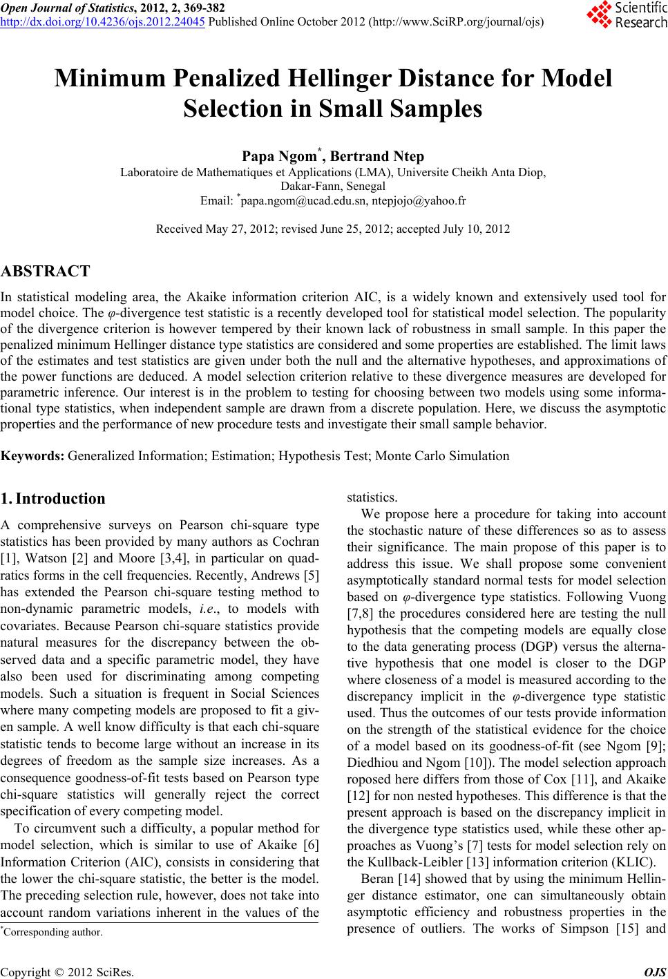
|