Wireless Sensor Network, 2010, 2, 606-611
doi:10.4236/wsn.2010.28072 Published Online August 2010 (http://www.SciRP.org/journal/wsn)
Distance Measurement Model Based on RSSI in WSN
Jiuqiang Xu, Wei Liu, Fenggao Lang, Yuanyuan Zhang, Chenglong Wang
School of Information Science & Engineering Northeastern University, Shenyang, China
Received May 18, 2010; revised June 9, 2010; accepted June 18, 2010
Abstract
The relationship between RSSI (Received Signal Strength Indication) values and distance is the foundation
and the key of ranging and positioning technologies in wireless sensor networks. Log-normal shadowing
model (LNSM), as a more general signal propagation model, can better describe the relationship between the
RSSI value and distance, but the parameter of variance in LNSM is depended on experiences without
self-adaptability. In this paper, it is found that the variance of RSSI value changes along with distance regu-
larly by analyzing a large number of experimental data. Based on the result of analysis, we proposed the re-
lationship function of the variance of RSSI and distance, and established the log-normal shadowing model
with dynamic variance (LNSM-DV). At the same time, the method of least squares(LS) was selected to es-
timate the coefficients in that model, thus LNSM-DV might be adjusted dynamically according to the change
of environment and be self-adaptable. The experimental results show that LNSM-DV can further reduce er-
ror, and have strong self-adaptability to various environments compared with the LNSM.
Keywords: WSN, Dynamic Variance, Distance Measurement, RSSI, Log-Normal Shadowing Model
1. Introduction
With the development of ranging and positioning tech-
nologies in wireless sensor networks(WSN) , it becomes
more and more important to find an mathematical model
which can accurately describe the relationship between
the RSSI [1] values and distance. This model should be
able to adjust parameters according to the change of en-
vironment by itself, and also be able to reduce error far-
thest.
Currently, there are three types of RSSI signal propa-
gation model for wireless sensor network (WSN),free
space model [2], 2-ray ground model [3] and log-normal
shadowing model (LNSM) [4]. The first two models
have special requirements for the application environ-
ment, while the third model is a more general signal
propagation model.
This paper, based on the studies of current RSSI
propagation models, with the goal of accuracy and self-
adaptability of model, we present a log-normal shadow-
ing model with the dynamic variance (LNSM-DV) and
establish the function of variance and distance. Using the
method of least squares(LS) to estimate parameters in the
model makes the parameters be able to be dynamically
adjusted according to the change of the environment, and
makes the model have self-adaptability. It has been veri-
fied by experiments that LNSM-DV can be further elimi-
nate errors and has a strong self-adaptability com- pared
with the original model. So LNSM-DV is able to more
accurately describe the relationship of the RSSI value
and the distance.
2. RSSI Ranging
RSSI, TOA [5], TDOA [6], and the AOA [7] are ranging
technologies commonly used now. Just as the use of
RSSI ranging need less communication overhead, lower
implementation complexity, and lower cost, so it is very
suitable for the nodes in wireless sensor network which
have limited power.
2.1. Principles of RSSI Ranging
The principle of RSSI ranging describes the relationship
between transmitted power and received power of wire-
less signals and the distance among nodes. This rela-
tionship is shown in (1). is the received power of
wireless signals. is the transmitted power of wireless
signal. is the distance between the sending nodes and
receiving nodes. is the transmission factor whose
value depends on the propagation environment.
r
P
t
P
n
d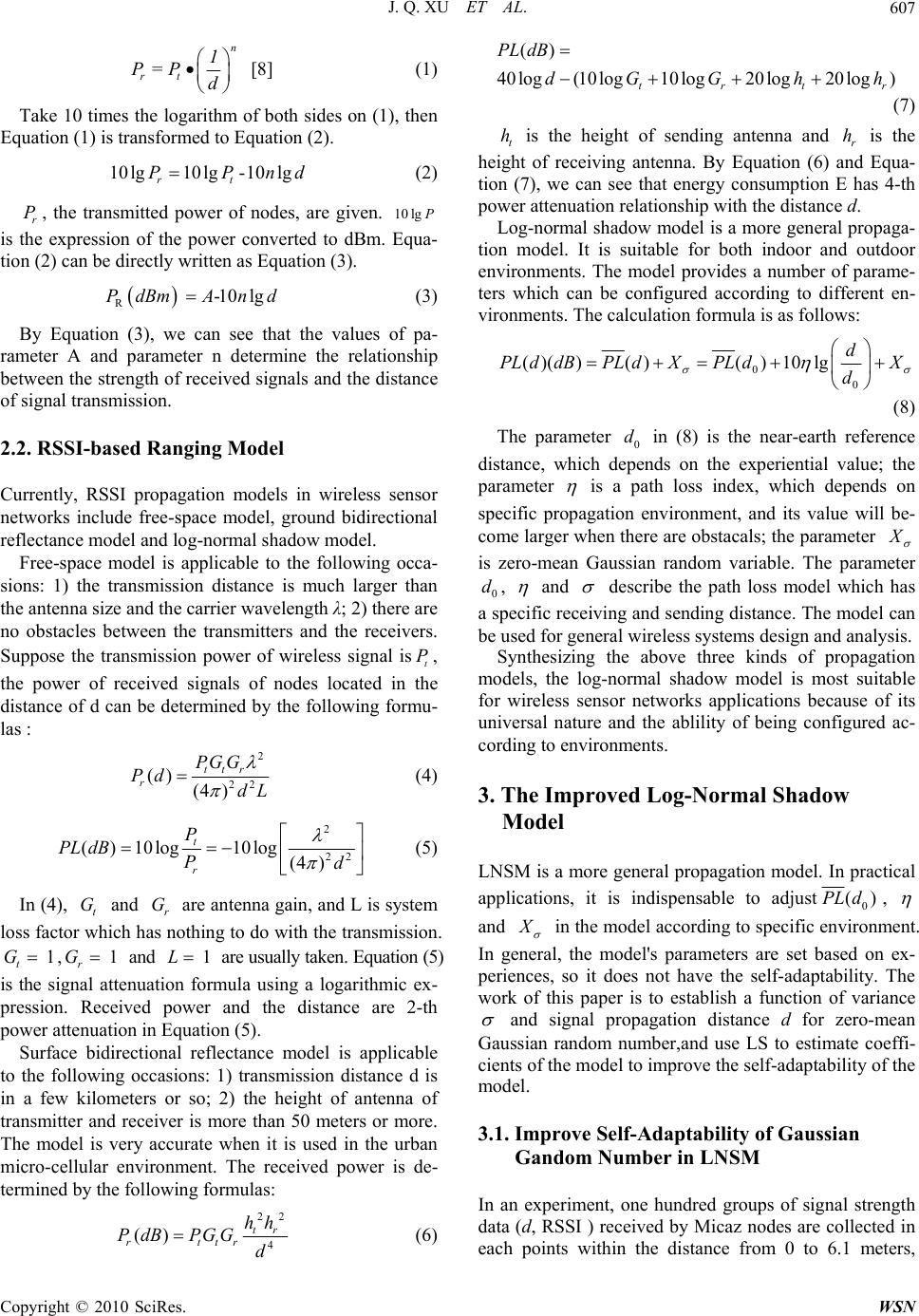

J. Q. XU ET AL.607
n
rt
1
P=P d



[8] (1)
Take 10 times the logarithm of both sides on (1), then
Equation (1) is transformed to Equation (2).
10 lg10 lg-10lg
rt
PPnd (2)
r
P, the transmitted power of nodes, are given.
is the expression of the power converted to dBm. Equa-
tion (2) can be directly written as Equation (3).
10 lgP

R-10 lgPdBmAn d (3)
By Equation (3), we can see that the values of pa-
rameter A and parameter n determine the relationship
between the strength of received signals and the distance
of signal transmission.
2.2. RSSI-based Ranging Model
Currently, RSSI propagation models in wireless sensor
networks include free-space model, ground bidirectional
reflectance model and log-normal shadow model.
Free-space model is applicable to the following occa-
sions: 1) the transmission distance is much larger than
the antenna size and the carrier wavelength λ; 2) there are
no obstacles between the transmitters and the receivers.
Suppose the transmission power of wireless signal is,
the power of received signals of nodes located in the
distance of d can be determined by the following formu-
las :
t
P
2
22
() (4 )
ttr
r
PG G
Pd dL


 (4)
2
22
()10log10 log(4 )
t
r
P
PL dBPd







(5)
In (4), and are antenna gain, and L is system
loss factor which has nothing to do with the transmission.
, and are usually taken. Equation (5)
is the signal attenuation formula using a logarithmic ex-
pression. Received power and the distance are 2-th
power attenuation in Equation (5).
t
G
r
G
r
G
L1
t
G11
Surface bidirectional reflectance model is applicable
to the following occasions: 1) transmission distance d is
in a few kilometers or so; 2) the height of antenna of
transmitter and receiver is more than 50 meters or more.
The model is very accurate when it is used in the urban
micro-cellular environment. The received power is de-
termined by the following formulas:
22
4
() tr
rttr
hh
PdBPGG d  (6)
()
40log(10log10log20log20log )
trt
PL dB
dGGh r h


(7)
t
h is the height of sending antenna and is the
height of receiving antenna. By Equation (6) and Equa-
tion (7), we can see that energy consumption E has 4-th
power attenuation relationship with the distance d.
r
h
Log-normal shadow model is a more general propaga-
tion model. It is suitable for both indoor and outdoor
environments. The model provides a number of parame-
ters which can be configured according to different en-
vironments. The calculation formula is as follows:
0
0
()()()() 10lgd PLd dBPLdXPLdX
d




 


 
(8)
The parameter in (8) is the near-earth reference
distance, which depends on the experiential value; the
parameter
0
d

is a path loss index, which depends on
specific propagation environment, and its value will be-
come larger when there are obstacals; the parameter
X

is zero-mean Gaussian random variable. The parameter
,
0
d

and

describe the path loss model which has
a specific receiving and sending distance. The model can
be used for general wireless systems design and analysis.
Synthesizing the above three kinds of propagation
models, the log-normal shadow model is most suitable
for wireless sensor networks applications because of its
universal nature and the ablility of being configured ac-
cording to environments.
3. The Improved Log-Normal Shadow
Model
LNSM is a more general propagation model. In practical
applications, it is indispensable to adjust0 ()PL d,

and
X

in the model according to specific environment.
In general, the model's parameters are set based on ex-
periences, so it does not have the self-adaptability. The
work of this paper is to establish a function of variance

and signal propagation distance d for zero-mean
Gaussian random number,and use LS to estimate coeffi-
cients of the model to improve the self-adaptability of the
model.
3.1. Improve Self-Adaptability of Gaussian
Gandom Number in LNSM
In an experiment, one hundred groups of signal strength
data (d, RSSI ) received by Micaz nodes are collected in
each points within the distance from 0 to 6.1 meters,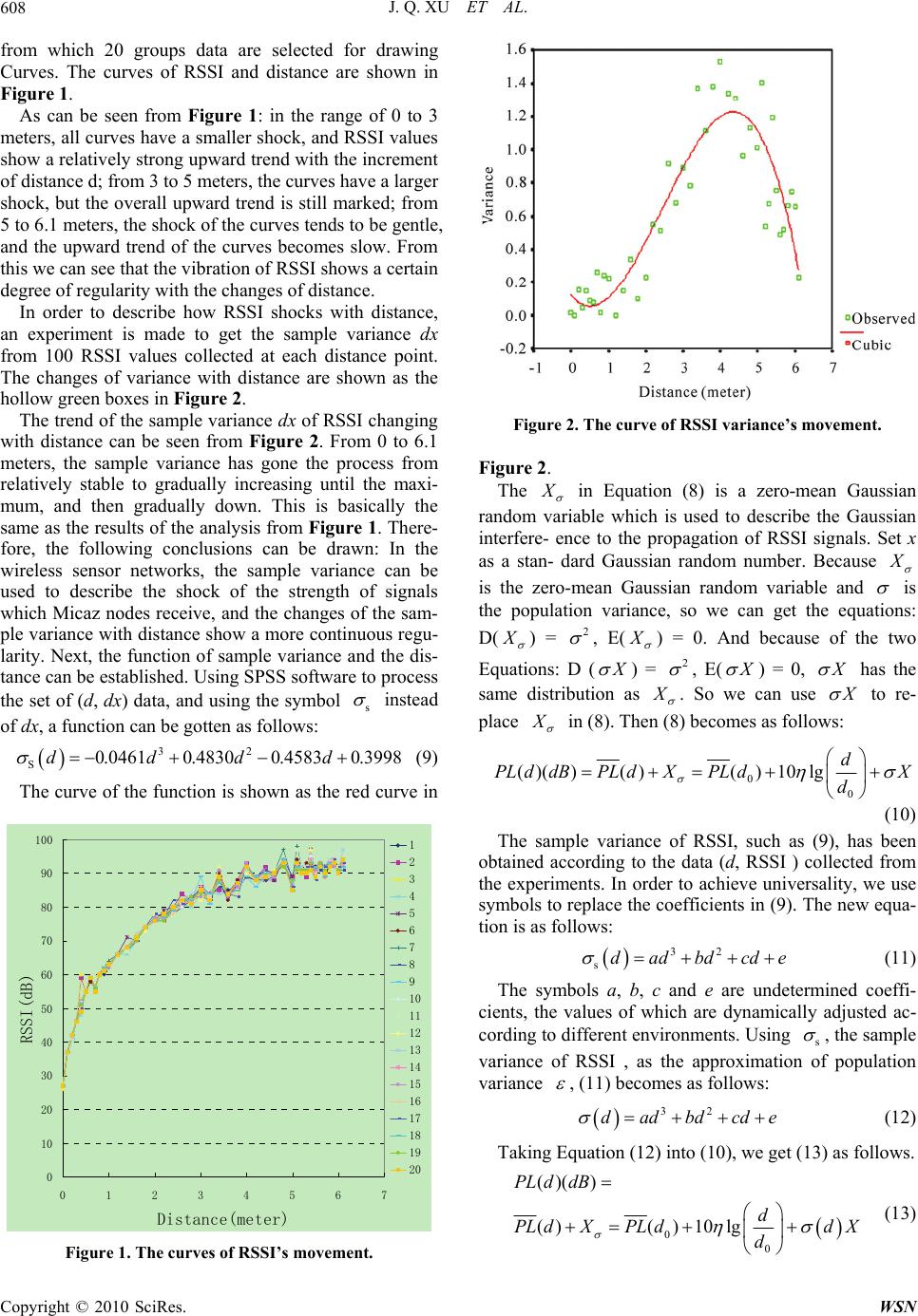

J. Q. XU ET AL. 608
from which 20 groups data are selected for drawing
Curves. The curves of RSSI and distance are shown in
Figure 1.
As can be seen from Figure 1: in the range of 0 to 3
meters, all curves have a smaller shock, and RSSI values
show a relatively strong upward trend with the increment
of distance d; from 3 to 5 meters, the curves have a larger
shock, but the overall upward trend is still marked; from
5 to 6.1 meters, the shock of the curves tends to be gentle,
and the upward trend of the curves becomes slow. From
this we can see that the vibration of RSSI shows a certain
degree of regularity with the changes of distance.
In order to describe how RSSI shocks with distance,
an experiment is made to get the sample variance dx
from 100 RSSI values collected at each distance point.
The changes of variance with distance are shown as the
hollow green boxes in Figure 2.
The trend of the sample variance dx of RSSI changing
with distance can be seen from Figure 2. From 0 to 6.1
meters, the sample variance has gone the process from
relatively stable to gradually increasing until the maxi-
mum, and then gradually down. This is basically the
same as the results of the analysis from Figure 1. There-
fore, the following conclusions can be drawn: In the
wireless sensor networks, the sample variance can be
used to describe the shock of the strength of signals
which Micaz nodes receive, and the changes of the sam-
ple variance with distance show a more continuous regu-
larity. Next, the function of sample variance and the dis-
tance can be established. Using SPSS software to process
the set of (d, dx) data, and using the symbol s

instead
of dx, a function can be gotten as follows:

32
S0.04610.48300.4583 0.3998dddd
  (9)
The curve of the function is shown as the red curve in
0
10
20
30
40
50
60
70
80
90
100
01234567
Distance(meter)
RSSI(dB)
1
2
3
4
5
6
7
8
9
10
11
12
13
14
15
16
17
18
19
20
Figure 1. The curves of RSSI’s movement.
Figure 2. The curve of RSSI variance’s movement.
Figure 2.
The
X

in Equation (8) is a zero-mean Gaussian
random variable which is used to describe the Gaussian
interfere- ence to the propagation of RSSI signals. Set x
as a stan- dard Gaussian random number. Because
X

is the zero-mean Gaussian random variable and

is
the population variance, so we can get the equations:
D(
X

) = 2

, E(
X

) = 0. And because of the two
Equations: D (
X

) = 2

, E(
X

) = 0,
X

has the
same distribution as
X

. So we can use
X

to re-
place
X

in (8). Then (8) becomes as follows:
0
0
()()()() 10lgd PLd dBPLdXPLdX
d




 


 
(10)
The sample variance of RSSI, such as (9), has been
obtained according to the data (d, RSSI ) collected from
the experiments. In order to achieve universality, we use
symbols to replace the coefficients in (9). The new equa-
tion is as follows:


32
sdadbdcd
 e

 (11)
The symbols a, b, c and e are undetermined coeffi-
cients, the values of which are dynamically adjusted ac-
cording to different environments. Using s

, the sample
variance of RSSI , as the approximation of population
variance

, (11) becomes as follows:


32
dadbdcd  e

 (12)
Taking Equation (12) into (10), we get (13) as follows.

0
0
()()
()() 10lg
PL ddB
d
PL dXPL ddX
d




 


  (13)

J. Q. XU ET AL.609
Equations (12) and (13) are the improved log-normal
shadow model. The establishment of the function


d 
makes LNSM be able to dynamically adjust the error
function according to the change of distance, which fur-
ther improves the ability to eliminate errors of the model.
3.2. The Realization of the Adaptability of
Coefficients in Log-Normal Shadow Model
The Self-adaptability of LNSM reflects not only in that
the variance of Gaussian function in LNSM could be
dynamically adjusted according to the changes of dis-
tance, but also in that the coefficients 0
()PL d,

, ,
, and could be dynamically adjusted according
to different environments. LS in regression analysis is
very suitable for estimating the coefficients in functions
because of its simplicity and its small amount of compu-
tation. The algorithm is derived as follows.
a
bc e
For convenience, change (13) to (14):
0
10 log()
d
rf d

   (14)
In (14), , ()()rPLddB()
f
PL d,


dX  ;
The parameter is the near-earth reference distance
that has already been known. Change (14) to (15):
0
d
0
10 log()
d
rf d    (15)
Then according to the principle of minimizing the sum
of error squares with LS, (16) is established as follows:

2
2
11 0
10 log()
nn i
ii
ii
d
Jrf
d







(16)
Calculate the partial derivative of
J
to

:
10
2010log()log()
nii
i
i
dd Jfr
dd







0
(17)
Let: 0
J


.Change (17) to (18):
2
111
00
10log( )log( )log( )0
nnn
ii
i
iii
ddd
fr
ddd






 0
i

(18)
In a similar way, calculate the partial derivative of
J
to
f
:
10
J210log()
ni
i
i
d
f
r
fd







(19)
Let: J0
f

. Change (19) to (20):
11
0
10 log()0
n
i
i
ii
dnf r
d



 



n

(20)
Thus, (18) and (20) constitute the linear simultaneous
equations on the coefficients (
f
,

) in (14), by which
the coefficients (
f
,

) can be solved.
Use to replace
y


d  in (12) and introduce ob-
servational errors

as follow.
32
yad bdcde


 (21)
Change (21) to (22).
32
y
adbdcde 

 (22)
Then according to the principle of minimizing the sum
of error squares with LS, (23) is established as follows:


22
32
11
nn
iiiii
ii
J
yad bd cde 


 (23)
Respectively calculate the partial derivative of
J
to
, , and and make them to 0, namely: abc e
0
J
a


, 0
J
b


, 0
J
c


, 0
J
e

. Thus, the linear
simultaneous equations on the coefficients (a､､ ､ )
are established as follows.
bc e
 
 
 


 
 
65433
11111
54322
11111
432
11111
32
111 1
0
0
0
0
nnnnn
iiiii
i
iiiii
nnnnn
iiii i
i
iiiii
nnnnn
iiii i
i
iiiii
nnn n
iii i
iii i
abce y
dddd d
abce y
dddd d
abce y
dddd d
abcney
ddd



 














 


 






(24)
Then the coefficients (a, b, c and e) can be solved by
(24).
In practice, when the experiment environments change,
the coefficients in (12) and (13) can be solved by (24)
and the linear simultaneous equations constituted by (18)
and (20). So LNSM-DV can be applied in different en-
vironments.
4. Experiment Analysis
4.1. Experiment Environment
Micaz nodes are used as the experimental hardware
platform, which are wireless sensor nodes produced by
Crossbow firm. Their communication module CC2420
has powerful communication capability. The core of the
node is Atmega128 that is a low-power, high-speed and
full-featured processor.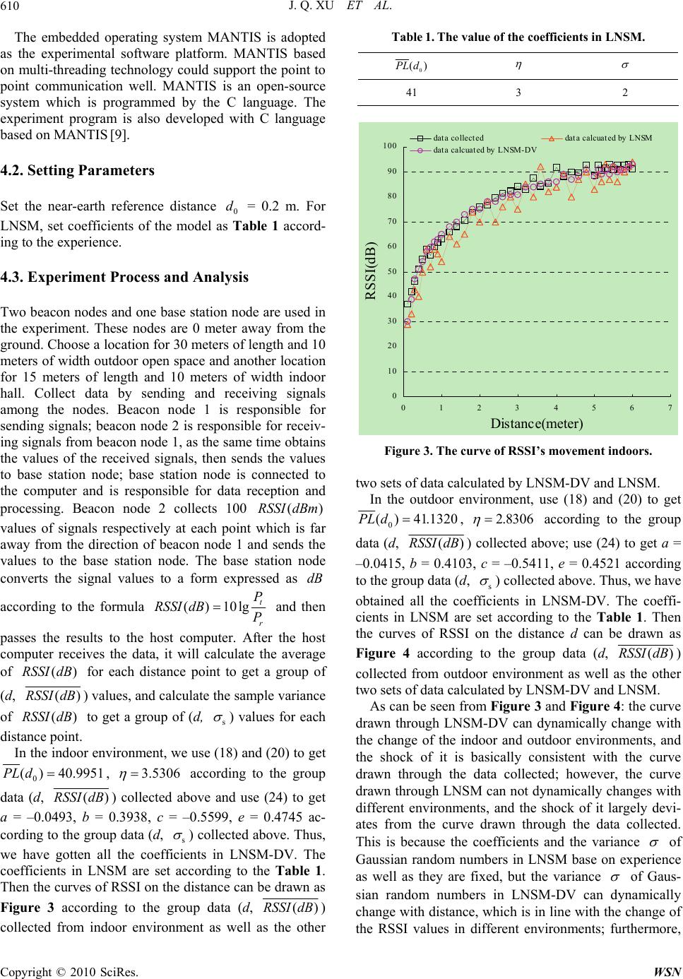

J. Q. XU ET AL. 610
The embedded operating system MANTIS is adopted
as the experimental software platform. MANTIS based
on multi-threading technology could support the point to
point communication well. MANTIS is an open-source
system which is programmed by the C language. The
experiment program is also developed with C language
based on MANTIS [9].
4.2. Setting Parameters
Set the near-earth reference distance = 0.2 m. For
LNSM, set coefficients of the model as Table 1 accord-
ing to the experience.
0
d
4.3. Experiment Process and Analysis
Two beacon nodes and one base station node are used in
the experiment. These nodes are 0 meter away from the
ground. Choose a location for 30 meters of length and 10
meters of width outdoor open space and another location
for 15 meters of length and 10 meters of width indoor
hall. Collect data by sending and receiving signals
among the nodes. Beacon node 1 is responsible for
sending signals; beacon node 2 is responsible for receiv-
ing signals from beacon node 1, as the same time obtains
the values of the received signals, then sends the values
to base station node; base station node is connected to
the computer and is responsible for data reception and
processing. Beacon node 2 collects 100
values of signals respectively at each point which is far
away from the direction of beacon node 1 and sends the
values to the base station node. The base station node
converts the signal values to a form expressed as
according to the formula
()RSSI dBm
dB
()10lg
t
r
P
P
RSSI dB and then
passes the results to the host computer. After the host
computer receives the data, it will calculate the average
of for each distance point to get a group of
(d,
()RSSI dB
()RSSI dB
()RSSI dB
) values, and calculate the sample variance
of to get a group of (d, s

) values for each
distance point.
In the indoor environment, we use (18) and (20) to get
0
( )40.9951PL d, 3.5306

 according to the group
data (d, ()
s
Table 1. The value of the coefficients in LNSM.
0
()PL d


41 3 2
0
10
20
30
40
50
60
70
80
90
100
01234567
Distance(meter)
RSSI(dB)
data collecteddata calcuated by LNSM
data calcuated by LNSM-DV
Figure 3. The curve of RSSI’s movement indoors.
two sets of data calculated by LNSM-DV and LNSM.
In the outdoor environment, use (18) and (20) to get
0
( )41.1320PLd, 2.8306


according to the group
data (d, ()
s
RSSI dB) collected above; use (24) to get a =
–0.0415, b = 0.4103, c = –0.5411, e = 0.4521 according
to the group data (d,

) collected above. Thus, we have
obtained all the coefficients in LNSM-DV. The coeffi-
cients in LNSM are set according to the Table 1. Then
the curves of RSSI on the distance d can be drawn as
Figure 4 according to the group data (d, ()RSSI dB)
collected from outdoor environment as well as the other
two sets of data calculated by LNSM-DV and LNSM.
As can be seen from Figure 3 and Figure 4: the curve
drawn through LNSM-DV can dynamically change with
the change of the indoor and outdoor environments, and
the shock of it is basically consistent with the curve
drawn through the data collected; however, the curve
drawn through LNSM can not dynamically changes with
different environments, and the shock of it largely devi-
ates from the curve drawn through the data collected.
This is because the coefficients and the variance

of
Gaussian random numbers in LNSM base on experience
as well as they are fixed, but the variance

of Gaus-
sian random numbers in LNSM-DV can dynamically
change with distance, which is in line with the change of
the RSSI values in different environments; furthermore,
RSSI dB) collected above and use (24) to get
a = –0.0493, b = 0.3938, c = –0.5599, e = 0.4745 ac-
cording to the group data (d,

) collected above. Thus,
we have gotten all the coefficients in LNSM-DV. The
coefficients in LNSM are set according to the Table 1.
Then the curves of RSSI on the distance can be drawn as
Figure 3 according to the group data (d, ()RSSIdB)
collected from indoor environment as well as the other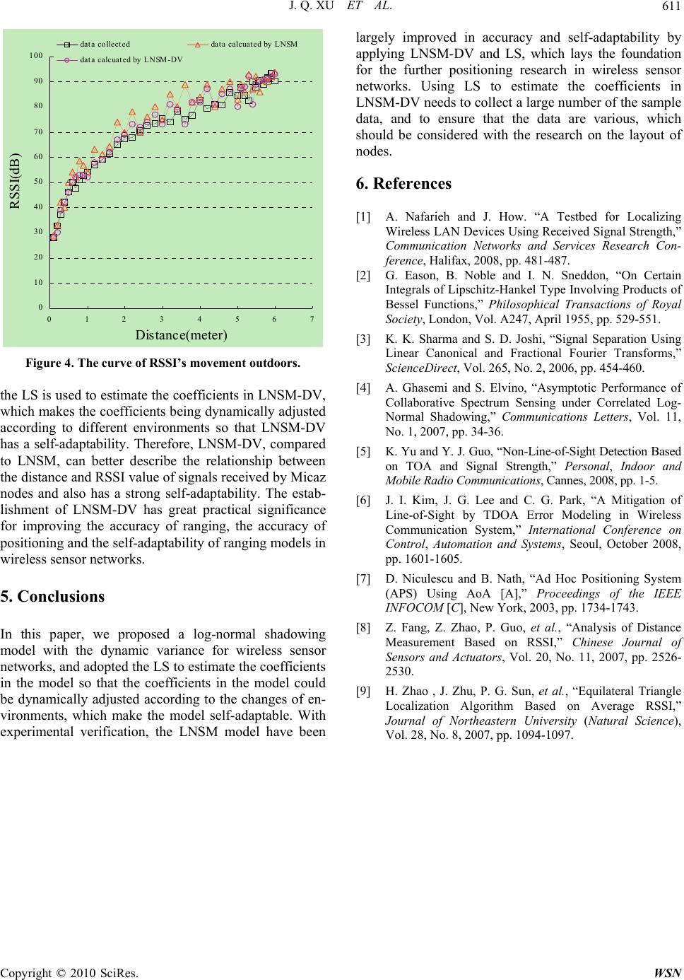

J. Q. XU ET AL. 611
0
10
20
30
40
50
60
70
80
90
100
01234567
Distance(meter)
RSSI(dB)
data collecteddata calcuated by LNSM
data calcuated by LNSM-DV
Figure 4. The curve of RSSI’s movement outdoors.
the LS is used to estimate the coefficients in LNSM-DV,
which makes the coefficients being dynamically adjusted
according to different environments so that LNSM-DV
has a self-adaptability. Therefore, LNSM-DV, compared
to LNSM, can better describe the relationship between
the distance and RSSI value of signals received by Micaz
nodes and also has a strong self-adaptability. The estab-
lishment of LNSM-DV has great practical significance
for improving the accuracy of ranging, the accuracy of
positioning and the self-adaptability of ranging models in
wireless sensor networks.
5. Conclusions
In this paper, we proposed a log-normal shadowing
model with the dynamic variance for wireless sensor
networks, and adopted the LS to estimate the coefficients
in the model so that the coefficients in the model could
be dynamically adjusted according to the changes of en-
vironments, which make the model self-adaptable. With
experimental verification, the LNSM model have been
largely improved in accuracy and self-adaptability by
applying LNSM-DV and LS, which lays the foundation
for the further positioning research in wireless sensor
networks. Using LS to estimate the coefficients in
LNSM-DV needs to collect a large number of the sample
data, and to ensure that the data are various, which
should be considered with the research on the layout of
nodes.
6. References
[1] A. Nafarieh and J. How. “A Testbed for Localizing
Wireless LAN Devices Using Received Signal Strength,”
Communication Networks and Services Research Con-
ference, Halifax, 2008, pp. 481-487.
[2] G. Eason, B. Noble and I. N. Sneddon, “On Certain
Integrals of Lipschitz-Hankel Type Involving Products of
Bessel Functions,” Philosophical Transactions of Royal
Society, London, Vol. A247, April 1955, pp. 529-551.
[3] K. K. Sharma and S. D. Joshi, “Signal Separation Using
Linear Canonical and Fractional Fourier Transforms,”
ScienceDirect, Vol. 265, No. 2, 2006, pp. 454-460.
[4] A. Ghasemi and S. Elvino, “Asymptotic Performance of
Collaborative Spectrum Sensing under Correlated Log-
Normal Shadowing,” Communications Letters, Vol. 11,
No. 1, 2007, pp. 34-36.
[5] K. Yu and Y. J. Guo, “Non-Line-of-Sight Detection Based
on TOA and Signal Strength,” Personal, Indoor and
Mobile Radio Communications, Cannes, 2008, pp. 1-5.
[6] J. I. Kim, J. G. Lee and C. G. Park, “A Mitigation of
Line-of-Sight by TDOA Error Modeling in Wireless
Communication System,” International Conference on
Control, Automation and Systems, Seoul, October 2008,
pp. 1601-1605.
[7] D. Niculescu and B. Nath, “Ad Hoc Positioning System
(APS) Using AoA [A],” Proceedings of the IEEE
INFOCOM [C], New York, 2003, pp. 1734-1743.
[8] Z. Fang, Z. Zhao, P. Guo, et al., “Analysis of Distance
Measurement Based on RSSI,” Chinese Journal of
Sensors and Actuators, Vol. 20, No. 11, 2007, pp. 2526-
2530.
[9] H. Zhao , J. Zhu, P. G. Sun, et al., “Equilateral Triangle
Localization Algorithm Based on Average RSSI,”
Journal of Northeastern University (Natural Science),
Vol. 28, No. 8, 2007, pp. 1094-1097.